
Supervised Instruction Fine-Tuning on Alpaca, Deployment, and Why 164M Isn’t Enough
In Part 7, I pretrained a 164M parameter GPT-style model (SydsGPTv2) on ~12B tokens using a carefully engineered pipeline on a single NVIDIA 3080 Ti. In this final part of the series, I shift from pure pretraining to instruction fine-tuning (SFT).
The goals for this phase were:
- Start from the pretrained SydsGPTv2 checkpoint.
- Fine-tune it on the Alpaca GPT-4 instruction dataset.
- Evaluate its instruction-following behavior.
- Deploy it via Hugging Face Hub + Gradio as a live demo.
- Reflect honestly on what a 164M parameter model can and cannot do in this regime.
I’ll walk through the full notebook: data download and formatting, dataset and dataloaders, collate function, model/optimizer setup, training loops, loss visualization, evaluation, and generation — including all code.
1. Setup: Imports and High-Level Workflow
This notebook is focused on fine-tuning, not pretraining. At a high level, the workflow is:
- Load and preprocess Alpaca.
- Tokenize and batch data for efficient training.
- Load the pretrained SydsGPTv2 model.
- Fine-tune with a warmup + cosine LR schedule and checkpointing.
- Visualize training/validation losses.
- Evaluate and generate outputs.
Basic PyTorch imports:
import torch
import torch.nn as nn
2. Downloading and Loading the Alpaca Dataset
I started by defining a small utility to download the dataset from a URL if it’s not already cached locally.
import json
import urllib
import os

def download_data(url, path):
    if not os.path.exists(path):
        with urllib.request.urlopen(url) as response:
            raw_data = response.read().decode('utf-8')
        with open(path, 'w', encoding = 'utf-8') as f:
            f.write(raw_data)
        print(f"Dataset downloaded and saved to {path}")
    else:
        print(f"Dataset already exists at {path}")

    with open(path, 'r') as f:
        data = json.load(f)
    return data
Then I downloaded and inspected the Alpaca GPT-4 data:
url = "https://raw.githubusercontent.com/Instruction-Tuning-with-GPT-4/GPT-4-LLM/refs/heads/main/data/alpaca_gpt4_data.json"
path = "data/alpaca_gpt4_data.json"
data = download_data(url, path)

print(f"Loaded {len(data)} records from the dataset.")
print("Sample record:", data[25])
3. Train/Test/Validation Split
I split the dataset into train, test, and validation:
- 85% train
- 10% test
- 5% validation
training_data = data[:int(len(data)*0.85)]
test_data = data[int(len(data)*0.85):int(len(data)*0.95)]
validation_data = data[int(len(data)*0.95):]

print(f"Training records: {len(training_data)}")
print(f"Test records: {len(test_data)}")
print(f"Validation records: {len(validation_data)}")
4. Formatting Records into Prompts
Instruction tuning lives and dies on the prompt format. For this, I used simple <|user|> and <|assistant|> tags.
Formatting a single Alpaca record into a user prompt:
def format_record(record):
    return f"<|user|>\n{record['instruction']}" + (f"\n{record['input']}" if record['input'] else "")
Example of combining prompt and response:
input = format_record(data[50])
response = f"\n\n<|assistant|>\n{data[50]['output']}"

print(input + response)
This is the core pattern used for training and evaluation.
5. Instruction Dataset: Encoding for SFT
I created a custom InstructionDataset that encodes <|user|> ... <|assistant|> ... pairs using tiktoken:
from torch.utils.data import Dataset

class InstructionDataset(Dataset):
    def __init__(self, data, tokenizer):
        self.data = data
        self.encoded_text = []
        for record in data:
            text = format_record(record) + f"\n\n<|assistant|>\n{record['output']}"
            self.encoded_text.append(tokenizer.encode(text))

    def __len__(self):
        return len(self.data)

    def __getitem__(self, idx):
        return self.encoded_text[idx]
6. Tokenizer Initialization and Padding Token
I reused the GPT-2 tokenizer from tiktoken and used its end-of-text token as padding:
import tiktoken
tokenizer = tiktoken.get_encoding("gpt2")
padding_token = tokenizer.eot_token
print(f"Padding token: {padding_token}")
7. Custom Collate Function for Instruction Batches
The collate function handles:
- Padding sequences in a batch to the maximum length.
- Creating input and target sequences shifted by one.
- Masking padding tokens in targets with an
ignore_idx(e.g.-100) so they don’t contribute to the loss. - Truncating to a fixed
context_size(2048). - Moving tensors to the correct device.
def instruction_collate_fn(batch, padding_token, ignore_idx, device, context_size):
    max_length = max(len(item) for item in batch)
    input_ids, target_ids = [], []

    for item in batch:
        padded_item = item + [padding_token] * (max_length - len(item))
        inputs = torch.tensor(padded_item)
        targets = torch.tensor(padded_item[1:] + [padding_token])
        mask = targets == padding_token
        idxs = torch.nonzero(mask).squeeze()
        if idxs.numel() > 1:
            targets[idxs[1:]] = ignore_idx

        if context_size is not None:
            inputs = inputs[:context_size]
            targets = targets[:context_size]

        input_ids.append(inputs)
        target_ids.append(targets)


    input_ids = torch.stack(input_ids).to(device)
    target_ids = torch.stack(target_ids).to(device)
    return input_ids, target_ids
I also sanity-checked the collate function with toy data:
test_inputs1 = [1,2,3,4,5,6,7,8]
test_inputs2 = [9,10,11]
test_inputs3 = [12,13,14,15]
batch = [test_inputs1, test_inputs2, test_inputs3]
padded_input_batch, padded_target_batch = instruction_collate_fn(batch, padding_token=padding_token, ignore_idx=-100, device='cpu', context_size=2048)
print(padded_input_batch)
print(padded_target_batch)
8. Device Selection
Standard GPU/CPU selection:
device = "cuda" if torch.cuda.is_available() else "cpu"
print(f"Using device: {device}")
9. DataLoaders for Train/Val/Test
I created a partial of the collate function with fixed parameters
from functools import partial
collate_fn = partial(instruction_collate_fn, padding_token=padding_token, ignore_idx=-100, device=device, context_size=2048)
Then set up dataloaders:
from torch.utils.data import DataLoader

num_workers = 0
batch_size = 2

train_dataset = InstructionDataset(training_data, tokenizer)
train_dataloader = DataLoader(train_dataset, batch_size = batch_size, collate_fn = collate_fn, num_workers = num_workers, shuffle = True, drop_last = True)

validation_dataset = InstructionDataset(validation_data, tokenizer)
validation_dataloader = DataLoader(validation_dataset, batch_size = batch_size, collate_fn = collate_fn, num_workers = num_workers, shuffle = False, drop_last = False)

test_dataset = InstructionDataset(test_data, tokenizer)
test_dataloader = DataLoader(test_dataset, batch_size = batch_size, collate_fn = collate_fn, num_workers = num_workers, shuffle = False, drop_last = False)
Quick inspection of shapes:
print("Train Loader:")
for i, (inputs, targets) in enumerate(train_dataloader):
    print(inputs.shape, targets.shape)
    if i == 4:
        break
10. Model Configuration and Initialization
I used the same configuration as in Part 7
SYDSGPT_CONFIG_V2_164M = {
    "vocab_size" : 50257,
    "context_length" : 2048,
    "embedding_dim" : 768,
    "num_heads" : 12,
    "num_layers" : 12,
    "dropout" : 0.1,
    "qkv_bias" : False
}
Then loaded the pretrained model and optimizer:
from galore_torch import GaLoreAdamW
from model.SydsGPTv2 import SydsGPTv2

model = SydsGPTv2(SYDSGPT_CONFIG_V2_164M)
model.load_state_dict(torch.load("sydsgpt/sydsgpt_v2_164m_trained_model-11.8B.pth", map_location=device))
optimizer = GaLoreAdamW(model.parameters(), weight_decay=0.01)
model.to(device)
11. Learning Rate Schedule: Warmup + Cosine
For fine-tuning I used small LRs
initial_lr = 5e-6
peak_lr = 2e-5
min_lr = 0.1 * peak_lr

print('Initial LR:', initial_lr)
print('Peak LR:', peak_lr)
print('Min LR:', min_lr)

total_steps_per_epoch = len(train_dataloader)
print('Total training steps per epoch:', total_steps_per_epoch)

warmup_steps = int(total_steps_per_epoch * .03)
print('Warmup steps:', warmup_steps)
The actual schedule logic lives in train_model_v2 (from modules.Training), which applies warmup then cosine decay over the total training horizon.
12. Fine-Tuning: First 2 Epochs
I kicked off the first stage of fine-tuning for 2 epochs
from modules.Training import train_model_v2

num_epochs = 2
training_losses, validation_losses, total_tokens_processed, learning_rates = train_model_v2(
    model,
    train_dataloader,
    validation_dataloader,
    optimizer,
    device,
    num_epochs,
    evaluation_frequency = 2000,
    start_context = format_record(validation_data[0]),
    tokenizer = tokenizer,
    checkpoint_interval = 2000,
    total_steps_per_epoch = total_steps_per_epoch,
    warmup_steps = warmup_steps,
    initial_lr = initial_lr,
    peak_lr = peak_lr,
    min_lr = min_lr
)
I saved the model after 2 epochs:
torch.save(model.state_dict(), "sydsgpt/sydsgpt_v2_164m_finetuned_alpaca_2epochs.pth")13. Extended Fine-Tuning: Up to 6 and 10 Epochs
Later, I saved a 6-epoch checkpoint:
torch.save(model.state_dict(), "sydsgpt/sydsgpt_v2_164m_finetuned_alpaca_6epochs.pth")Then I reinitialized the optimizer and trained for 4 more epochs (total 10):
from galore_torch import GaLoreAdamW
optimizer = GaLoreAdamW(model.parameters(), weight_decay=0.01)
from modules.Training import train_model_v2
num_epochs = 4
training_losses, validation_losses, total_tokens_processed, learning_rates = train_model_v2(
model,
train_dataloader,
validation_dataloader,
optimizer,
device,
num_epochs,
evaluation_frequency = 2000,
start_context = format_record(validation_data[0]),
tokenizer = tokenizer,
checkpoint_interval = 2000,
total_steps_per_epoch = total_steps_per_epoch,
warmup_steps = warmup_steps,
initial_lr = initial_lr,
peak_lr = peak_lr,
min_lr = min_lr
)And saved the 10-epoch checkpoint:
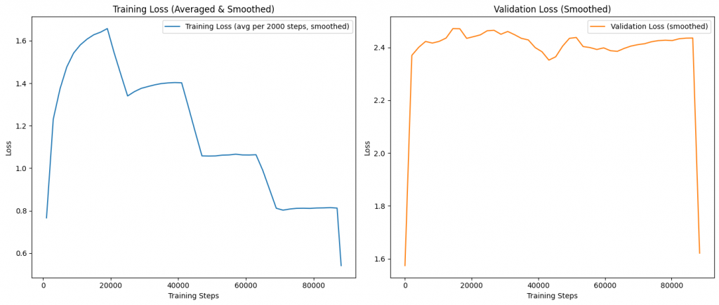
torch.save(model.state_dict(), "sydsgpt/sydsgpt_v2_164m_finetuned_alpaca_10epochs.pth")14. Visualizing Training and Validation Loss
I used the same plotting pattern twice (after 6 and after 10 epochs) to visualize loss:

import numpy as np
from matplotlib import pyplot as plt
# Concatenate losses and tokens across both training runs
train_loss = training_losses
val_loss = validation_losses
# Build step indices for raw series
steps = np.arange(1, len(train_loss) + 1)
# Simple moving average smoothing
def smooth_series(y, window=101):
if len(y) < 3:
return np.array(y)
# Choose an odd window <= len(y)
w = min(window, max(3, (len(y) // 50) * 2 + 1))
if w % 2 == 0:
w += 1
kernel = np.ones(w) / w
return np.convolve(y, kernel, mode='same')
# Average training loss every 2000 steps
bin_size = 2000
num_bins = int(np.ceil(len(train_loss) / bin_size))
train_bins = [
np.mean(train_loss[i * bin_size : (i + 1) * bin_size])
for i in range(num_bins)
]
# Use bin midpoints for x-axis
bin_steps = np.array([
int(min(((i * bin_size) + min(len(train_loss), (i + 1) * bin_size)) // 2, len(train_loss)))
for i in range(num_bins)
])
# Smooth the binned training loss for nicer curves
train_binned_smooth = smooth_series(np.array(train_bins), window=min(21, len(train_bins) if len(train_bins) > 0 else 21))
# Smooth validation loss (keep at per-step resolution)
val_smooth = smooth_series(np.array(val_loss))
# Create side-by-side subplots: training (binned + smoothed) and validation
fig, axs = plt.subplots(1, 2, figsize=(14, 6), sharex=False)
# Left: Training loss averages (smoothed)
ax1 = axs[0]
ax1.plot(bin_steps, train_binned_smooth, label='Training Loss (avg per 2000 steps, smoothed)', color='tab:blue')
ax1.set_xlabel('Training Steps')
ax1.set_ylabel('Loss')
ax1.set_title('Training Loss (Averaged & Smoothed)')
ax1.legend(loc='upper right')
# Right: Validation loss (smoothed) on its own
val_steps = np.linspace(1, len(train_loss), len(val_smooth), dtype=int)
ax2 = axs[1]
ax2.plot(val_steps, val_smooth, label='Validation Loss (smoothed)', color='tab:orange')
ax2.set_xlabel('Training Steps')
ax2.set_ylabel('Loss')
ax2.set_title('Validation Loss (Smoothed)')
ax2.legend(loc='upper right')
plt.tight_layout()
plt.show()15. Final Validation Loss Evaluation
I computed the final validation loss over all batches after 6 and 10 epochs using calc_loader_loss:
from modules.Loss import calc_loader_loss
final_validation_loss = calc_loader_loss(validation_dataloader, model, device, num_batches=len(validation_dataloader))
print(f"Final Validation Loss after 6 epochs (All batches): {final_validation_loss:.4f}")And again after 10 epochs:
from modules.Loss import calc_loader_loss
final_validation_loss = calc_loader_loss(validation_dataloader, model, device, num_batches=len(validation_dataloader))
print(f"Final Validation Loss after 10 epochs (All batches): {final_validation_loss:.4f}")The Validation loss was better after 6 epochs than after 10 epochs, so i decided to proceed with the 6 epochs model for the next steps.
16. Loading the Fine-Tuned Model for Evaluation
To evaluate, I reloaded the fine-tuned model
from model.SydsGPTv2 import SydsGPTv2
device = torch.device('cuda' if torch.cuda.is_available() else 'cpu')
print(f"Using device: {device}")
model = SydsGPTv2(SYDSGPT_CONFIG_V2_164M)
model.load_state_dict(torch.load("sydsgpt/sydsgpt_v2_164m_finetuned_alpaca_6epochs.pth", map_location=device))
model.to(device)17. Generating and Evaluating Responses on Test Data
I generated responses on the first five test examples
from modules.Generate import text_to_tokens, tokens_to_text, generate
for record in test_data[:5]:
input_text = format_record(record)
print(f"Input Text:\n{input_text.replace("<|user|>", "")}")
input_tokens = text_to_tokens(input_text, tokenizer).to(device)
output_tokens = generate(
model,
input_tokens,
max_new_tokens = 200,
context_size = 2048,
temperature = 0.7,
top_k = 40,
eos_id = tokenizer.eot_token
)
output_text = tokens_to_text(output_tokens, tokenizer)
response_text = output_text[len(input_text):].replace("<|assistant|>", "").strip()
print(f"Model Response:\n{response_text}")
print(f"Correct Response:\n{record['output']}")This qualitative comparison was key for understanding how well the model was actually following instructions, beyond loss curves.
18. Custom Prompt Generation
I also tried a custom instruction:
from modules.Generate import text_to_tokens, tokens_to_text, generate
model.eval()
input_text = """<|user|>
give me exactly 3 different sentences about the earth."""
print(f"Input Text:\n{input_text.replace("<|user|>", "")}")
input_tokens = text_to_tokens(input_text, tokenizer).to(device)
output_tokens = generate(
model,
input_tokens,
max_new_tokens = 200,
context_size = 2048,
temperature = 0.7,
top_k = 40,
eos_id = tokenizer.eot_token
)
output_text = tokens_to_text(output_tokens, tokenizer)
response_text = output_text[len(input_text):].replace("<|assistant|>", "").strip()
print(f"Model Response:\n{response_text}")This is the kind of prompt that reveals adherence to constraints (e.g., “exactly 3 sentences”) — something small models often struggle with.
19. Deployment: Hugging Face Model + Gradio Space
From here, I:
- Uploaded
sydsgpt_v2_164m_finetuned_alpaca_6epochs.pth(and later 10 epochs) to Hugging Face as a model repo. - Wrapped the model in a Gradio app hosted on Hugging Face Spaces to demo interactive instruction-following.
You can check out the running demo here: Sydsgpt V2 165M SFT Demo – a Hugging Face Space by siddsachar
The model can follow basic instructions, respond sensibly, and display some generalization. But it quickly showed its limits: shallow reasoning, inconsistent adherence to constraints, and occasional drift in longer responses.
20. Honest Reflection: 164M Parameters Are Not Enough
This is the crux of Part 8.
After multiple epochs of fine-tuning, careful LR scheduling, and qualitative evaluation via a live demo, the conclusion was clear:
A 164M parameter GPT-style model has insufficient capacity for robust, high-quality instruction following — at least with this approach and this dataset.
It’s a strong teaching model, a great vehicle for learning and documentation, and a very capable toy. But as an instruction follower, it falls short of what we’ve come to expect from modern assistants.
And that’s okay — that was part of the experiment.
21. Where I’m Going Next
This is the final part of this series, but not the end of the project.
Next steps will focus on:
- Scaling capacity:
Expanding the base model to ~500M parameters while reusing as much of the existing training pipeline as possible. - LoRA-based specialization:
Adding LoRA adapters for:- Instruction following
- Summarization
- Q&A
- And later, tool use and RAG
- Multi-adapter design:
Exploring how to route between different adapters and capabilities without retraining the entire base model. - Tool use and RAG:
Giving the model structured access to tools and a retrieval layer so it can ground its outputs in external knowledge.
Try It Yourself
The full notebook with all the steps, from preparing the corpus, data loaders, loss computation, pretraining loop, text sampling and generation, is available here:
SydsGPT ALPACA SFT Repository
Clone the repo, open the Jupyter notebook, and step through the code.
Build It Yourself
If you want to try building it yourself, you can find the complete code with detailed explanations of each block in the source code section at the end of this post. All the best!
Closing the Series
This series was never just about “getting a model to work.” It was about:
- Understanding pretraining end-to-end on modest hardware.
- Building a data + model + training pipeline from scratch.
- Documenting the process so others can reproduce and adapt it.
- Testing the boundary of what a small, self-hostable model can do.
Instruction fine-tuning on Alpaca — and deploying the result — was the last major piece. It showed the limits of 164M, and in doing so, set the direction for what comes next.
The next chapter won’t be called “from scratch” anymore. It’ll be about scaling, modularity, and practical alignment.
Source Code
Model Training and Evaluation Workflow
This notebook demonstrates the process of fine-tuning a GPT-style language model on the Alpaca dataset using PyTorch. The workflow includes:
- Loading and preprocessing the Alpaca dataset.
- Tokenizing and batching data for efficient training.
- Defining and initializing the SydsGPTv2 model.
- Training the model with custom learning rate scheduling and checkpointing.
- Visualizing training and validation loss curves.
- Evaluating the model’s performance on validation data.
- Generating sample outputs from the fine-tuned model.
The following code cell loads the necessary PyTorch modules and defines the model and optimizer for training. The model is loaded from a pre-trained checkpoint and moved to the appropriate device (CPU or GPU) for computation. The optimizer used is GaLoreAdamW, which is suitable for large language models.
Key steps in the code cell:
- Importing the
GaLoreAdamWoptimizer and theSydsGPTv2model class. - Setting the device to CUDA if available, otherwise CPU.
- Initializing the model with the specified configuration.
- Loading pre-trained model weights from a checkpoint file.
- Initializing the optimizer with model parameters and weight decay.
- Moving the model to the selected device.
This setup prepares the model and optimizer for the subsequent training and evaluation steps.
import torch
import torch.nn as nn
Data Download and Preparation
This code cell defines a utility function for downloading and loading the Alpaca dataset from a remote URL. The function, download_data, checks if the dataset already exists locally at the specified path. If not, it downloads the dataset using urllib, saves it as a JSON file, and then loads it into memory. If the file already exists, it skips the download and directly loads the data. This ensures efficient data management and avoids redundant downloads. The function returns the loaded dataset as a Python object for further processing.
import json
import urllib
import os
def download_data(url, path):
if not os.path.exists(path):
with urllib.request.urlopen(url) as response:
raw_data = response.read().decode('utf-8')
with open(path, 'w', encoding = 'utf-8') as f:
f.write(raw_data)
print(f"Dataset downloaded and saved to {path}")
else:
print(f"Dataset already exists at {path}")
with open(path, 'r') as f:
data = json.load(f)
return data
Downloading and Loading the Alpaca Dataset
The following code cell downloads the Alpaca dataset from a specified remote URL and loads it into memory for further processing. The download_data function checks if the dataset already exists locally at the given path. If the file does not exist, it downloads the dataset using urllib, saves it as a JSON file, and then loads it. If the file is already present, it skips the download and loads the data directly from disk. This approach ensures efficient data management and avoids redundant downloads. The loaded dataset is returned as a Python object for subsequent preprocessing and analysis.
Key steps in the code cell:
- Define the remote URL and local file path for the dataset.
- Use the
download_datafunction to download and load the dataset. - Print the number of records loaded and display a sample record for inspection.
url = "https://raw.githubusercontent.com/Instruction-Tuning-with-GPT-4/GPT-4-LLM/refs/heads/main/data/alpaca_gpt4_data.json"
path = "data/alpaca_gpt4_data.json"
data = download_data(url, path)
print(f"Loaded {len(data)} records from the dataset.")
print("Sample record:", data[25])
Dataset already exists at data/alpaca_gpt4_data.json
Loaded 52002 records from the dataset.
Sample record: {'instruction': 'Explain the concept of cogging torque.', 'input': '', 'output': "Cogging torque is a torque that's produced by the interaction between the magnetic field of the stator (the stationary component in an electric motor or generator) and the rotor (the rotating component). This interaction produces a magnetic attraction between the stator teeth and the rotor poles. This scenario leads to an uneven torque, which makes the motor to experience a jerky motion instead of smooth rotation.\n\nCogging torque is mainly experienced in motors with a large number of turns in the rotor and stator windings and when the motor has a small air gap. The cogging effect can be reduced by skewing the stator or rotor slots or by choosing the number of stator and rotor slots accordingly. A proper design reduces the cogging torque, thus resulting in smooth and continuous rotation."}
Formatting a Single Alpaca Record for Model Input
The following code cell defines a utility function, format_record, which takes a single record from the Alpaca dataset and formats it into a prompt suitable for GPT-style language models. The function constructs the prompt by including the instruction and, if present, the input field from the record. The formatted prompt begins with a special <|user|> token, followed by the instruction, and appends the input on a new line if it exists. This formatting is essential for consistent model training and inference, ensuring that the model receives inputs in the expected structure.
Key points:
- The function handles records with or without an input field.
- The output string is ready to be concatenated with the assistant’s response for supervised fine-tuning.
- This utility is used throughout the notebook for preparing both training and evaluation data.
def format_record(record):
return f"<|user|>\n{record['instruction']}" + (f"\n{record['input']}" if record['input'] else "")
Formatting and Displaying a Sample Alpaca Record
This code cell demonstrates how to format a single record from the Alpaca dataset into a prompt suitable for GPT-style language models and display both the formatted input and the expected assistant response. The process involves:
- Selecting a specific record from the loaded dataset (in this case, record at index 50).
- Using the
format_recordutility function to convert the record’s instruction and input fields into a standardized prompt format, beginning with the<|user|>token. - Appending the assistant’s response, prefixed by the
<|assistant|>token, to the formatted prompt. - Printing the complete prompt and response, which can be used for model training or inspection.
This step is useful for verifying the formatting logic and inspecting how the data will be presented to the model during supervised fine-tuning.
input = format_record(data[50])
response = f"\n\n<|assistant|>\n{data[50]['output']}"
print(input + response)
<|user|> Edit the following sentence to make it more concise. He ran to the bus stop in order to catch the bus that was due to arrive in five minutes. <|assistant|> He ran to the bus stop to catch the arriving bus in five minutes.
Splitting the Alpaca Dataset into Training, Test, and Validation Sets
This code cell divides the loaded Alpaca dataset into three distinct subsets for model development:
- Training Set (85%): Used to train the model and update its parameters.
- Test Set (10%): Used to evaluate the model’s performance during development and tune hyperparameters.
- Validation Set (5%): Used for final evaluation to assess the model’s generalization ability after training.
The dataset is split by slicing the list of records according to the specified proportions. The code prints the number of records in each subset to verify the split.
training_data = data[:int(len(data)*0.85)]
test_data = data[int(len(data)*0.85):int(len(data)*0.95)]
validation_data = data[int(len(data)*0.95):]
print(f"Training records: {len(training_data)}")
print(f"Test records: {len(test_data)}")
print(f"Validation records: {len(validation_data)}")
Training records: 44201 Test records: 5200 Validation records: 2601
Creating a PyTorch Dataset for Instruction Tuning
The following code cell defines a custom PyTorch Dataset class, InstructionDataset, tailored for instruction tuning with the Alpaca dataset. This dataset class is responsible for:
- Initialization: Accepts a list of data records and a tokenizer. For each record, it formats the instruction and output using the
format_recordfunction, appends the assistant’s response, and encodes the combined text into token IDs using the provided tokenizer. - Length: Returns the total number of records in the dataset.
- Item Retrieval: Provides access to the encoded token sequence for a given index, enabling efficient batching and sampling during training.
This dataset class is essential for preparing data in a format compatible with PyTorch’s DataLoader, facilitating efficient mini-batch training of language models on instruction-following tasks.
from torch.utils.data import Dataset
class InstructionDataset(Dataset):
def __init__(self, data, tokenizer):
self.data = data
self.encoded_text = []
for record in data:
text = format_record(record) + f"\n\n<|assistant|>\n{record['output']}"
self.encoded_text.append(tokenizer.encode(text))
def __len__(self):
return len(self.data)
def __getitem__(self, idx):
return self.encoded_text[idx]
Tokenizer Initialization and Padding Token Selection
This code cell initializes the tokenizer required for encoding and decoding text data for the GPT-style model. It uses the tiktoken library to load the GPT-2 tokenizer, which is compatible with the model architecture. The cell also retrieves the special end-of-text (EOT) token from the tokenizer, which will be used as the padding token during batching and sequence alignment. The padding token ensures that all sequences in a batch have the same length, which is necessary for efficient processing in PyTorch. The selected padding token is printed for verification.
Key steps:
- Import the
tiktokenlibrary. - Load the GPT-2 tokenizer using
tiktoken.get_encoding("gpt2"). - Retrieve the EOT token from the tokenizer and assign it as the padding token.
- Print the padding token for confirmation.
import tiktoken
tokenizer = tiktoken.get_encoding("gpt2")
padding_token = tokenizer.eot_token
print(f"Padding token: {padding_token}")
Padding token: 50256
Custom Collate Function for Instruction Tuning Batches
This code cell defines the instruction_collate_fn, a custom collate function for batching sequences in instruction tuning tasks. The function is designed to:
- Pad sequences: Each sequence in the batch is padded to the length of the longest sequence using the specified
padding_token. - Prepare input and target tensors: For each sequence, the function creates input and target tensors. The target tensor is shifted by one position to align with the next-token prediction objective.
- Mask padding tokens: All padding tokens in the target tensor are masked with
ignore_idx(except the first occurrence), ensuring that loss computation ignores these positions. - Truncate to context size: If a
context_sizeis specified, both input and target tensors are truncated to this maximum length. - Move tensors to device: The resulting input and target tensors are stacked and moved to the specified device (CPU or GPU).
This collate function is essential for preparing batches compatible with language model training, ensuring correct padding, masking, and device placement.
def instruction_collate_fn(batch, padding_token, ignore_idx, device, context_size):
max_length = max(len(item) for item in batch)
input_ids, target_ids = [], []
for item in batch:
padded_item = item + [padding_token] * (max_length - len(item))
inputs = torch.tensor(padded_item)
targets = torch.tensor(padded_item[1:] + [padding_token])
mask = targets == padding_token
idxs = torch.nonzero(mask).squeeze()
if idxs.numel() > 1:
targets[idxs[1:]] = ignore_idx
if context_size is not None:
inputs = inputs[:context_size]
targets = targets[:context_size]
input_ids.append(inputs)
target_ids.append(targets)
input_ids = torch.stack(input_ids).to(device)
target_ids = torch.stack(target_ids).to(device)
return input_ids, target_ids
Testing the Custom Collate Function for Batching
This code cell demonstrates how to use the instruction_collate_fn function to batch and pad sequences for instruction tuning. Three example input sequences of varying lengths are created and combined into a batch. The custom collate function is then called with the batch, the selected padding token, an ignore index for masked positions, the device (cpu), and a context size of 2048 tokens.
Key steps:
- Define three test input sequences of different lengths.
- Combine them into a batch list.
- Call
instruction_collate_fnto pad the sequences and generate input and target tensors. - Print the resulting padded input and target tensors to verify correct padding and masking.
This test ensures that the collate function correctly handles variable-length sequences, applies padding, and prepares the data for model training.
test_inputs1 = [1,2,3,4,5,6,7,8]
test_inputs2 = [9,10,11]
test_inputs3 = [12,13,14,15]
batch = [test_inputs1, test_inputs2, test_inputs3]
padded_input_batch, padded_target_batch = instruction_collate_fn(batch, padding_token=padding_token, ignore_idx=-100, device='cpu', context_size=2048)
print(padded_input_batch)
print(padded_target_batch)
tensor([[ 1, 2, 3, 4, 5, 6, 7, 8],
[ 9, 10, 11, 50256, 50256, 50256, 50256, 50256],
[ 12, 13, 14, 15, 50256, 50256, 50256, 50256]])
tensor([[ 2, 3, 4, 5, 6, 7, 8, 50256],
[ 10, 11, 50256, -100, -100, -100, -100, -100],
[ 13, 14, 15, 50256, -100, -100, -100, -100]])
Device Selection for Model Training and Inference
This code cell determines the appropriate device (GPU or CPU) for running model computations using PyTorch. It checks if CUDA-enabled GPUs are available and sets the device variable accordingly. Using a GPU can significantly accelerate training and inference for deep learning models. The selected device is printed for confirmation.
Key steps:
- Use
torch.cuda.is_available()to check for GPU availability. - Set the
devicevariable to"cuda"if a GPU is available, otherwise"cpu". - Print the selected device for user awareness.
device = "cuda" if torch.cuda.is_available() else "cpu"
print(f"Using device: {device}")
Using device: cuda
Creating DataLoaders for Training, Validation, and Testing
This code cell constructs PyTorch DataLoader objects for the training, validation, and test splits of the Alpaca dataset. The InstructionDataset class is used to wrap each data split, encoding the records using the initialized tokenizer. The custom collate_fn ensures that batches are properly padded and formatted for instruction tuning.
Key steps:
- Set the number of worker processes (
num_workers) and batch size (batch_size). - Instantiate
InstructionDatasetfor each data split: training, validation, and test. - Create
DataLoaderobjects for each dataset, specifying batch size, custom collate function, shuffling, and whether to drop the last incomplete batch. - The resulting DataLoaders enable efficient mini-batch loading and preprocessing during model training and evaluation.
from functools import partial
collate_fn = partial(instruction_collate_fn, padding_token=padding_token, ignore_idx=-100, device=device, context_size=2048)
from torch.utils.data import DataLoader
num_workers = 0
batch_size = 2
train_dataset = InstructionDataset(training_data, tokenizer)
train_dataloader = DataLoader(train_dataset, batch_size = batch_size, collate_fn = collate_fn, num_workers = num_workers, shuffle = True, drop_last = True)
validation_dataset = InstructionDataset(validation_data, tokenizer)
validation_dataloader = DataLoader(validation_dataset, batch_size = batch_size, collate_fn = collate_fn, num_workers = num_workers, shuffle = False, drop_last = False)
test_dataset = InstructionDataset(test_data, tokenizer)
test_dataloader = DataLoader(test_dataset, batch_size = batch_size, collate_fn = collate_fn, num_workers = num_workers, shuffle = False, drop_last = False)
Inspecting the Structure of the Training DataLoader
This code cell provides a quick inspection of the batches produced by the train_dataloader. It iterates through the first few batches and prints the shapes of the input and target tensors. This is useful for verifying that the batching, padding, and collation logic are functioning as expected. By examining the tensor shapes, you can confirm that each batch has the correct dimensions (batch size, sequence length) and that the data is ready for model training.
Key steps:
- Iterate over the
train_dataloaderusing a loop. - For each batch, print the shapes of the input and target tensors.
- Limit the output to the first five batches for concise inspection.
print("Train Loader:")
for i, (inputs, targets) in enumerate(train_dataloader):
print(inputs.shape, targets.shape)
if i == 4:
break
Train Loader: torch.Size([8, 548]) torch.Size([8, 548]) torch.Size([8, 249]) torch.Size([8, 249]) torch.Size([8, 288]) torch.Size([8, 288]) torch.Size([8, 328]) torch.Size([8, 328]) torch.Size([8, 399]) torch.Size([8, 399])
SydsGPTv2 Model Configuration
This code cell defines the configuration dictionary for the SydsGPTv2 language model, specifically the 164M parameter variant. The configuration includes key architectural hyperparameters required to instantiate the model:
- vocab_size: The size of the tokenizer vocabulary (number of unique tokens the model can handle).
- context_length: The maximum sequence length (number of tokens) the model can process in a single forward pass.
- embedding_dim: The dimensionality of the token embeddings and hidden states.
- num_heads: The number of attention heads in each transformer layer.
- num_layers: The total number of transformer layers (depth of the model).
- dropout: The dropout probability used for regularization within the model.
- qkv_bias: Whether to include a bias term in the query, key, and value projections of the attention mechanism.
This configuration dictionary is used when initializing the SydsGPTv2 model to ensure consistency and reproducibility across training and evaluation runs.
SYDSGPT_CONFIG_V2_164M = {
"vocab_size" : 50257,
"context_length" : 2048,
"embedding_dim" : 768,
"num_heads" : 12,
"num_layers" : 12,
"dropout" : 0.1,
"qkv_bias" : False
}
Model and Optimizer Initialization
This code cell sets up the SydsGPTv2 language model and its optimizer for fine-tuning on the Alpaca dataset. The following steps are performed:
- Importing Required Modules: The
GaLoreAdamWoptimizer is imported for efficient training of large language models, and theSydsGPTv2model class is imported for model instantiation. - Device Selection: The code automatically selects a GPU (
cuda) if available, otherwise defaults to the CPU, ensuring optimal computation speed. - Model Initialization: The SydsGPTv2 model is instantiated using the predefined configuration dictionary
SYDSGPT_CONFIG_V2_164M, which specifies the model architecture. - Loading Pre-trained Weights: The model’s parameters are loaded from a checkpoint file, allowing for continued training or evaluation from a previously saved state.
- Optimizer Setup: The
GaLoreAdamWoptimizer is initialized with the model’s parameters and a specified weight decay for regularization. - Model to Device: The model is moved to the selected device (GPU or CPU) to prepare for training or inference.
This initialization is a crucial step before starting the training loop, ensuring that the model and optimizer are correctly configured and ready for efficient computation.
from galore_torch import GaLoreAdamW
from model.SydsGPTv2 import SydsGPTv2
device = torch.device('cuda' if torch.cuda.is_available() else 'cpu')
print(f"Using device: {device}")
model = SydsGPTv2(SYDSGPT_CONFIG_V2_164M)
model.load_state_dict(torch.load("sydsgpt/sydsgpt_v2_164m_trained_model-11.8B.pth", map_location=device))
optimizer = GaLoreAdamW(model.parameters(), weight_decay=0.01)
model.to(device)
e:\Code\SydsGPT-FineTuning\.venv\Lib\site-packages\tqdm\auto.py:21: TqdmWarning: IProgress not found. Please update jupyter and ipywidgets. See https://ipywidgets.readthedocs.io/en/stable/user_install.html from .autonotebook import tqdm as notebook_tqdm
Using device: cuda
e:\Code\SydsGPT-FineTuning\.venv\Lib\site-packages\galore_torch\adamw.py:48: FutureWarning: This implementation of AdamW is deprecated and will be removed in a future version. Use the PyTorch implementation torch.optim.AdamW instead, or set `no_deprecation_warning=True` to disable this warning warnings.warn(
SydsGPTv2(
(token_embedding): Embedding(50257, 768)
(position_embedding): Embedding(2048, 768)
(drop_embedding): Dropout(p=0.1, inplace=False)
(transformer_blocks): Sequential(
(0): TransformerBlockv2(
(attention): FlashAttention(
(qkv): Linear(in_features=768, out_features=2304, bias=True)
(out_proj): Linear(in_features=768, out_features=768, bias=True)
)
(layer_norm1): LayerNorm()
(feed_forward): FeedForward(
(layers): Sequential(
(0): Linear(in_features=768, out_features=3072, bias=True)
(1): GELU()
(2): Linear(in_features=3072, out_features=768, bias=True)
)
)
(layer_norm2): LayerNorm()
(dropout): Dropout(p=0.1, inplace=False)
)
(1): TransformerBlockv2(
(attention): FlashAttention(
(qkv): Linear(in_features=768, out_features=2304, bias=True)
(out_proj): Linear(in_features=768, out_features=768, bias=True)
)
(layer_norm1): LayerNorm()
(feed_forward): FeedForward(
(layers): Sequential(
(0): Linear(in_features=768, out_features=3072, bias=True)
(1): GELU()
(2): Linear(in_features=3072, out_features=768, bias=True)
)
)
(layer_norm2): LayerNorm()
(dropout): Dropout(p=0.1, inplace=False)
)
(2): TransformerBlockv2(
(attention): FlashAttention(
(qkv): Linear(in_features=768, out_features=2304, bias=True)
(out_proj): Linear(in_features=768, out_features=768, bias=True)
)
(layer_norm1): LayerNorm()
(feed_forward): FeedForward(
(layers): Sequential(
(0): Linear(in_features=768, out_features=3072, bias=True)
(1): GELU()
(2): Linear(in_features=3072, out_features=768, bias=True)
)
)
(layer_norm2): LayerNorm()
(dropout): Dropout(p=0.1, inplace=False)
)
(3): TransformerBlockv2(
(attention): FlashAttention(
(qkv): Linear(in_features=768, out_features=2304, bias=True)
(out_proj): Linear(in_features=768, out_features=768, bias=True)
)
(layer_norm1): LayerNorm()
(feed_forward): FeedForward(
(layers): Sequential(
(0): Linear(in_features=768, out_features=3072, bias=True)
(1): GELU()
(2): Linear(in_features=3072, out_features=768, bias=True)
)
)
(layer_norm2): LayerNorm()
(dropout): Dropout(p=0.1, inplace=False)
)
(4): TransformerBlockv2(
(attention): FlashAttention(
(qkv): Linear(in_features=768, out_features=2304, bias=True)
(out_proj): Linear(in_features=768, out_features=768, bias=True)
)
(layer_norm1): LayerNorm()
(feed_forward): FeedForward(
(layers): Sequential(
(0): Linear(in_features=768, out_features=3072, bias=True)
(1): GELU()
(2): Linear(in_features=3072, out_features=768, bias=True)
)
)
(layer_norm2): LayerNorm()
(dropout): Dropout(p=0.1, inplace=False)
)
(5): TransformerBlockv2(
(attention): FlashAttention(
(qkv): Linear(in_features=768, out_features=2304, bias=True)
(out_proj): Linear(in_features=768, out_features=768, bias=True)
)
(layer_norm1): LayerNorm()
(feed_forward): FeedForward(
(layers): Sequential(
(0): Linear(in_features=768, out_features=3072, bias=True)
(1): GELU()
(2): Linear(in_features=3072, out_features=768, bias=True)
)
)
(layer_norm2): LayerNorm()
(dropout): Dropout(p=0.1, inplace=False)
)
(6): TransformerBlockv2(
(attention): FlashAttention(
(qkv): Linear(in_features=768, out_features=2304, bias=True)
(out_proj): Linear(in_features=768, out_features=768, bias=True)
)
(layer_norm1): LayerNorm()
(feed_forward): FeedForward(
(layers): Sequential(
(0): Linear(in_features=768, out_features=3072, bias=True)
(1): GELU()
(2): Linear(in_features=3072, out_features=768, bias=True)
)
)
(layer_norm2): LayerNorm()
(dropout): Dropout(p=0.1, inplace=False)
)
(7): TransformerBlockv2(
(attention): FlashAttention(
(qkv): Linear(in_features=768, out_features=2304, bias=True)
(out_proj): Linear(in_features=768, out_features=768, bias=True)
)
(layer_norm1): LayerNorm()
(feed_forward): FeedForward(
(layers): Sequential(
(0): Linear(in_features=768, out_features=3072, bias=True)
(1): GELU()
(2): Linear(in_features=3072, out_features=768, bias=True)
)
)
(layer_norm2): LayerNorm()
(dropout): Dropout(p=0.1, inplace=False)
)
(8): TransformerBlockv2(
(attention): FlashAttention(
(qkv): Linear(in_features=768, out_features=2304, bias=True)
(out_proj): Linear(in_features=768, out_features=768, bias=True)
)
(layer_norm1): LayerNorm()
(feed_forward): FeedForward(
(layers): Sequential(
(0): Linear(in_features=768, out_features=3072, bias=True)
(1): GELU()
(2): Linear(in_features=3072, out_features=768, bias=True)
)
)
(layer_norm2): LayerNorm()
(dropout): Dropout(p=0.1, inplace=False)
)
(9): TransformerBlockv2(
(attention): FlashAttention(
(qkv): Linear(in_features=768, out_features=2304, bias=True)
(out_proj): Linear(in_features=768, out_features=768, bias=True)
)
(layer_norm1): LayerNorm()
(feed_forward): FeedForward(
(layers): Sequential(
(0): Linear(in_features=768, out_features=3072, bias=True)
(1): GELU()
(2): Linear(in_features=3072, out_features=768, bias=True)
)
)
(layer_norm2): LayerNorm()
(dropout): Dropout(p=0.1, inplace=False)
)
(10): TransformerBlockv2(
(attention): FlashAttention(
(qkv): Linear(in_features=768, out_features=2304, bias=True)
(out_proj): Linear(in_features=768, out_features=768, bias=True)
)
(layer_norm1): LayerNorm()
(feed_forward): FeedForward(
(layers): Sequential(
(0): Linear(in_features=768, out_features=3072, bias=True)
(1): GELU()
(2): Linear(in_features=3072, out_features=768, bias=True)
)
)
(layer_norm2): LayerNorm()
(dropout): Dropout(p=0.1, inplace=False)
)
(11): TransformerBlockv2(
(attention): FlashAttention(
(qkv): Linear(in_features=768, out_features=2304, bias=True)
(out_proj): Linear(in_features=768, out_features=768, bias=True)
)
(layer_norm1): LayerNorm()
(feed_forward): FeedForward(
(layers): Sequential(
(0): Linear(in_features=768, out_features=3072, bias=True)
(1): GELU()
(2): Linear(in_features=3072, out_features=768, bias=True)
)
)
(layer_norm2): LayerNorm()
(dropout): Dropout(p=0.1, inplace=False)
)
)
(final_layer_norm): LayerNorm()
(output_projection): Linear(in_features=768, out_features=50257, bias=False)
)
Learning Rate Schedule and Training Step Calculation
This code cell sets up the learning rate schedule and calculates the number of training steps per epoch for the fine-tuning process. It defines the initial, peak, and minimum learning rates, which are used to control the optimizer’s step size during training. The cell also computes the total number of training steps in each epoch based on the size of the training DataLoader. Additionally, it determines the number of warmup steps, which is a small fraction (3%) of the total steps per epoch, during which the learning rate will gradually increase from the initial to the peak value. These parameters are essential for implementing advanced learning rate scheduling strategies, such as warmup and decay, to improve model convergence and stability.
Key steps:
- Define initial, peak, and minimum learning rates.
- Calculate the total number of training steps per epoch.
- Compute the number of warmup steps as 3% of the total steps.
- Print all calculated values for verification.
initial_lr = 5e-6
peak_lr = 2e-5
min_lr = 0.1 * peak_lr
print('Initial LR:', initial_lr)
print('Peak LR:', peak_lr)
print('Min LR:', min_lr)
total_steps_per_epoch = len(train_dataloader)
print('Total training steps per epoch:', total_steps_per_epoch)
warmup_steps = int(total_steps_per_epoch * .03)
print('Warmup steps:', warmup_steps)
Initial LR: 5e-06 Peak LR: 2e-05 Min LR: 2.0000000000000003e-06 Total training steps per epoch: 22100 Warmup steps: 663
Training the Model for 2 Epochs
This code cell initiates the fine-tuning process of the SydsGPTv2 language model on the Alpaca dataset for 2 epochs. The training is performed using the train_model_v2 function, which handles the training loop, periodic evaluation, learning rate scheduling, and checkpointing. Key parameters and steps include:
- Model and Optimizer: The pre-initialized SydsGPTv2 model and GaLoreAdamW optimizer are used for training.
- DataLoaders: The training and validation DataLoaders provide mini-batches of tokenized and padded data.
- Device: Training is performed on the selected device (GPU or CPU).
- Epochs: The model is trained for 2 complete passes over the training data.
- Evaluation Frequency: Validation loss is computed every 2000 training steps to monitor progress.
- Learning Rate Schedule: The learning rate is managed with warmup and decay phases, using the specified initial, peak, and minimum values.
- Checkpointing: Model checkpoints are saved every 2000 steps for recovery and analysis.
- Start Context: A formatted prompt from the validation set is used as the initial context for evaluation.
- Outputs: The function returns lists of training and validation losses, the total number of tokens processed, and the learning rates used during training.
This cell is essential for launching the main training loop and tracking the model’s learning progress over time.
from modules.Training import train_model_v2
num_epochs = 2
training_losses, validation_losses, total_tokens_processed, learning_rates = train_model_v2(
model,
train_dataloader,
validation_dataloader,
optimizer,
device,
num_epochs,
evaluation_frequency = 2000,
start_context = format_record(validation_data[0]),
tokenizer = tokenizer,
checkpoint_interval = 2000,
total_steps_per_epoch = total_steps_per_epoch,
warmup_steps = warmup_steps,
initial_lr = initial_lr,
peak_lr = peak_lr,
min_lr = min_lr
)
Saving the Fine-Tuned Model Checkpoint
This code cell saves the current state of the fine-tuned SydsGPTv2 model to disk after completing 2 epochs of training on the Alpaca dataset. Saving model checkpoints is essential for:
- Reproducibility: Allows you to reload the exact model weights for future inference or continued training.
- Experiment Tracking: Enables comparison between different training runs or hyperparameter settings.
- Recovery: Protects against data loss in case of interruptions during long training sessions.
The model’s parameters are saved using PyTorch’s torch.save() function, which serializes the model’s state dictionary to the specified file path. This checkpoint can later be loaded with model.load_state_dict() for evaluation or further fine-tuning.
torch.save(model.state_dict(), "sydsgpt/sydsgpt_v2_164m_finetuned_alpaca_2epochs.pth")
Saving the Fine-Tuned Model Checkpoint After 6 Epochs
This code cell saves the state dictionary of the SydsGPTv2 model after completing 6 epochs of fine-tuning on the Alpaca dataset.
torch.save(model.state_dict(), "sydsgpt/sydsgpt_v2_164m_finetuned_alpaca_6epochs.pth")
Training and Validation Loss Visualization
This code cell visualizes the training and validation loss curves over the course of model fine-tuning. Effective visualization helps in diagnosing model convergence, overfitting, and generalization performance. The cell performs the following steps:
- Imports: Loads
numpyandmatplotlib.pyplotfor numerical operations and plotting. - Loss Preparation: Uses the
training_lossesandvalidation_losseslists, which contain the per-step loss values recorded during training and validation. - Smoothing: Defines a
smooth_seriesfunction to apply a moving average, reducing noise in the loss curves for clearer trends. - Binning: Averages the training loss every 2000 steps to match the evaluation frequency and reduce plot clutter.
- Plotting:
- The left subplot displays the smoothed, binned training loss.
- The right subplot shows the smoothed validation loss.
- Both plots use appropriate axis labels, titles, and legends for clarity.
- Layout: Uses
plt.tight_layout()to ensure the subplots are neatly arranged.
This visualization provides insights into the model’s learning dynamics and helps identify issues such as underfitting, overfitting, or learning rate problems.
import numpy as np
from matplotlib import pyplot as plt
# Concatenate losses and tokens across both training runs
train_loss = training_losses
val_loss = validation_losses
# Build step indices for raw series
steps = np.arange(1, len(train_loss) + 1)
# Simple moving average smoothing
def smooth_series(y, window=101):
if len(y) < 3:
return np.array(y)
# Choose an odd window <= len(y)
w = min(window, max(3, (len(y) // 50) * 2 + 1))
if w % 2 == 0:
w += 1
kernel = np.ones(w) / w
return np.convolve(y, kernel, mode='same')
# Average training loss every 2000 steps
bin_size = 2000
num_bins = int(np.ceil(len(train_loss) / bin_size))
train_bins = [
np.mean(train_loss[i * bin_size : (i + 1) * bin_size])
for i in range(num_bins)
]
# Use bin midpoints for x-axis
bin_steps = np.array([
int(min(((i * bin_size) + min(len(train_loss), (i + 1) * bin_size)) // 2, len(train_loss)))
for i in range(num_bins)
])
# Smooth the binned training loss for nicer curves
train_binned_smooth = smooth_series(np.array(train_bins), window=min(21, len(train_bins) if len(train_bins) > 0 else 21))
# Smooth validation loss (keep at per-step resolution)
val_smooth = smooth_series(np.array(val_loss))
# Create side-by-side subplots: training (binned + smoothed) and validation
fig, axs = plt.subplots(1, 2, figsize=(14, 6), sharex=False)
# Left: Training loss averages (smoothed)
ax1 = axs[0]
ax1.plot(bin_steps, train_binned_smooth, label='Training Loss (avg per 2000 steps, smoothed)', color='tab:blue')
ax1.set_xlabel('Training Steps')
ax1.set_ylabel('Loss')
ax1.set_title('Training Loss (Averaged & Smoothed)')
ax1.legend(loc='upper right')
# Right: Validation loss (smoothed) on its own
val_steps = np.linspace(1, len(train_loss), len(val_smooth), dtype=int)
ax2 = axs[1]
ax2.plot(val_steps, val_smooth, label='Validation Loss (smoothed)', color='tab:orange')
ax2.set_xlabel('Training Steps')
ax2.set_ylabel('Loss')
ax2.set_title('Validation Loss (Smoothed)')
ax2.legend(loc='upper right')
plt.tight_layout()
plt.show()

Final Validation Loss Evaluation After 6 Epochs
This code cell evaluates the fine-tuned SydsGPTv2 model’s performance on the entire validation set after 6 epochs of training. It uses the calc_loader_loss function to compute the average loss across all batches in the validation_dataloader. This provides a quantitative measure of how well the model generalizes to unseen data after extended fine-tuning. The resulting validation loss is printed with four decimal places for clarity.
Key steps:
- Import the
calc_loader_lossutility from themodules.Lossmodule. - Compute the average validation loss over all batches.
- Print the final validation loss for reference and comparison.
from modules.Loss import calc_loader_loss
final_validation_loss = calc_loader_loss(validation_dataloader, model, device, num_batches=len(validation_dataloader))
print(f"Final Validation Loss after 6 epochs (All batches): {final_validation_loss:.4f}")
Final Validation Loss after 6 epochs (All batches): 2.1810
Loading and Evaluating the Fine-Tuned SydsGPTv2 Model
This code cell demonstrates how to load the SydsGPTv2 language model from a checkpoint after 6 epochs of fine-tuning on the Alpaca dataset and evaluate its performance on a subset of the test data. The workflow includes:
- Model Loading: The SydsGPTv2 model is instantiated with the correct configuration and its weights are loaded from the checkpoint file
"sydsgpt/sydsgpt_v2_164m_finetuned_alpaca_6epochs.pth". The model is moved to the appropriate device (GPU or CPU) for inference. - Text Generation: For each of the first five records in the test set, the input prompt is formatted using the
format_recordfunction. The prompt is tokenized and passed to the model’sgeneratefunction, which produces a response using autoregressive decoding with specified parameters (maximum new tokens, context size, temperature, top-k sampling, and end-of-sequence token). - Output Decoding and Display: The generated tokens are decoded back to text, and the assistant’s response is extracted and printed alongside the original prompt and the correct reference output from the dataset.
This evaluation provides a qualitative assessment of the model’s instruction-following capabilities after fine-tuning, allowing you to compare the generated responses with the ground-truth answers.
from model.SydsGPTv2 import SydsGPTv2
device = torch.device('cuda' if torch.cuda.is_available() else 'cpu')
print(f"Using device: {device}")
model = SydsGPTv2(SYDSGPT_CONFIG_V2_164M)
model.load_state_dict(torch.load("sydsgpt/sydsgpt_v2_164m_finetuned_alpaca_6epochs.pth", map_location=device))
model.to(device)
Using device: cuda
SydsGPTv2(
(token_embedding): Embedding(50257, 768)
(position_embedding): Embedding(2048, 768)
(drop_embedding): Dropout(p=0.1, inplace=False)
(transformer_blocks): Sequential(
(0): TransformerBlockv2(
(attention): FlashAttention(
(qkv): Linear(in_features=768, out_features=2304, bias=True)
(out_proj): Linear(in_features=768, out_features=768, bias=True)
)
(layer_norm1): LayerNorm()
(feed_forward): FeedForward(
(layers): Sequential(
(0): Linear(in_features=768, out_features=3072, bias=True)
(1): GELU()
(2): Linear(in_features=3072, out_features=768, bias=True)
)
)
(layer_norm2): LayerNorm()
(dropout): Dropout(p=0.1, inplace=False)
)
(1): TransformerBlockv2(
(attention): FlashAttention(
(qkv): Linear(in_features=768, out_features=2304, bias=True)
(out_proj): Linear(in_features=768, out_features=768, bias=True)
)
(layer_norm1): LayerNorm()
(feed_forward): FeedForward(
(layers): Sequential(
(0): Linear(in_features=768, out_features=3072, bias=True)
(1): GELU()
(2): Linear(in_features=3072, out_features=768, bias=True)
)
)
(layer_norm2): LayerNorm()
(dropout): Dropout(p=0.1, inplace=False)
)
(2): TransformerBlockv2(
(attention): FlashAttention(
(qkv): Linear(in_features=768, out_features=2304, bias=True)
(out_proj): Linear(in_features=768, out_features=768, bias=True)
)
(layer_norm1): LayerNorm()
(feed_forward): FeedForward(
(layers): Sequential(
(0): Linear(in_features=768, out_features=3072, bias=True)
(1): GELU()
(2): Linear(in_features=3072, out_features=768, bias=True)
)
)
(layer_norm2): LayerNorm()
(dropout): Dropout(p=0.1, inplace=False)
)
(3): TransformerBlockv2(
(attention): FlashAttention(
(qkv): Linear(in_features=768, out_features=2304, bias=True)
(out_proj): Linear(in_features=768, out_features=768, bias=True)
)
(layer_norm1): LayerNorm()
(feed_forward): FeedForward(
(layers): Sequential(
(0): Linear(in_features=768, out_features=3072, bias=True)
(1): GELU()
(2): Linear(in_features=3072, out_features=768, bias=True)
)
)
(layer_norm2): LayerNorm()
(dropout): Dropout(p=0.1, inplace=False)
)
(4): TransformerBlockv2(
(attention): FlashAttention(
(qkv): Linear(in_features=768, out_features=2304, bias=True)
(out_proj): Linear(in_features=768, out_features=768, bias=True)
)
(layer_norm1): LayerNorm()
(feed_forward): FeedForward(
(layers): Sequential(
(0): Linear(in_features=768, out_features=3072, bias=True)
(1): GELU()
(2): Linear(in_features=3072, out_features=768, bias=True)
)
)
(layer_norm2): LayerNorm()
(dropout): Dropout(p=0.1, inplace=False)
)
(5): TransformerBlockv2(
(attention): FlashAttention(
(qkv): Linear(in_features=768, out_features=2304, bias=True)
(out_proj): Linear(in_features=768, out_features=768, bias=True)
)
(layer_norm1): LayerNorm()
(feed_forward): FeedForward(
(layers): Sequential(
(0): Linear(in_features=768, out_features=3072, bias=True)
(1): GELU()
(2): Linear(in_features=3072, out_features=768, bias=True)
)
)
(layer_norm2): LayerNorm()
(dropout): Dropout(p=0.1, inplace=False)
)
(6): TransformerBlockv2(
(attention): FlashAttention(
(qkv): Linear(in_features=768, out_features=2304, bias=True)
(out_proj): Linear(in_features=768, out_features=768, bias=True)
)
(layer_norm1): LayerNorm()
(feed_forward): FeedForward(
(layers): Sequential(
(0): Linear(in_features=768, out_features=3072, bias=True)
(1): GELU()
(2): Linear(in_features=3072, out_features=768, bias=True)
)
)
(layer_norm2): LayerNorm()
(dropout): Dropout(p=0.1, inplace=False)
)
(7): TransformerBlockv2(
(attention): FlashAttention(
(qkv): Linear(in_features=768, out_features=2304, bias=True)
(out_proj): Linear(in_features=768, out_features=768, bias=True)
)
(layer_norm1): LayerNorm()
(feed_forward): FeedForward(
(layers): Sequential(
(0): Linear(in_features=768, out_features=3072, bias=True)
(1): GELU()
(2): Linear(in_features=3072, out_features=768, bias=True)
)
)
(layer_norm2): LayerNorm()
(dropout): Dropout(p=0.1, inplace=False)
)
(8): TransformerBlockv2(
(attention): FlashAttention(
(qkv): Linear(in_features=768, out_features=2304, bias=True)
(out_proj): Linear(in_features=768, out_features=768, bias=True)
)
(layer_norm1): LayerNorm()
(feed_forward): FeedForward(
(layers): Sequential(
(0): Linear(in_features=768, out_features=3072, bias=True)
(1): GELU()
(2): Linear(in_features=3072, out_features=768, bias=True)
)
)
(layer_norm2): LayerNorm()
(dropout): Dropout(p=0.1, inplace=False)
)
(9): TransformerBlockv2(
(attention): FlashAttention(
(qkv): Linear(in_features=768, out_features=2304, bias=True)
(out_proj): Linear(in_features=768, out_features=768, bias=True)
)
(layer_norm1): LayerNorm()
(feed_forward): FeedForward(
(layers): Sequential(
(0): Linear(in_features=768, out_features=3072, bias=True)
(1): GELU()
(2): Linear(in_features=3072, out_features=768, bias=True)
)
)
(layer_norm2): LayerNorm()
(dropout): Dropout(p=0.1, inplace=False)
)
(10): TransformerBlockv2(
(attention): FlashAttention(
(qkv): Linear(in_features=768, out_features=2304, bias=True)
(out_proj): Linear(in_features=768, out_features=768, bias=True)
)
(layer_norm1): LayerNorm()
(feed_forward): FeedForward(
(layers): Sequential(
(0): Linear(in_features=768, out_features=3072, bias=True)
(1): GELU()
(2): Linear(in_features=3072, out_features=768, bias=True)
)
)
(layer_norm2): LayerNorm()
(dropout): Dropout(p=0.1, inplace=False)
)
(11): TransformerBlockv2(
(attention): FlashAttention(
(qkv): Linear(in_features=768, out_features=2304, bias=True)
(out_proj): Linear(in_features=768, out_features=768, bias=True)
)
(layer_norm1): LayerNorm()
(feed_forward): FeedForward(
(layers): Sequential(
(0): Linear(in_features=768, out_features=3072, bias=True)
(1): GELU()
(2): Linear(in_features=3072, out_features=768, bias=True)
)
)
(layer_norm2): LayerNorm()
(dropout): Dropout(p=0.1, inplace=False)
)
)
(final_layer_norm): LayerNorm()
(output_projection): Linear(in_features=768, out_features=50257, bias=False)
)
Generating and Evaluating Model Responses on Test Data
This code cell demonstrates how to generate responses from the fine-tuned SydsGPTv2 model on the first five examples of the test set and compare them to the ground-truth outputs. The workflow includes:
- Prompt Formatting: For each test record, the input is formatted using the
format_recordfunction to match the expected prompt structure for the model. - Tokenization: The formatted prompt is tokenized using the
text_to_tokensutility and moved to the appropriate device (CPU or GPU). - Autoregressive Generation: The model generates a response using the
generatefunction, which performs autoregressive decoding with specified parameters such as maximum new tokens, context size, temperature, top-k sampling, and the end-of-sequence token. - Decoding and Extraction: The generated tokens are decoded back to text using
tokens_to_text, and the assistant’s response is extracted by removing the prompt and special tokens. - Comparison and Display: The input prompt, model-generated response, and the correct reference output are printed for each example, allowing for qualitative assessment of the model’s instruction-following capabilities.
This evaluation provides insight into how well the model generalizes to unseen instructions and how closely its outputs match the expected answers.
from modules.Generate import text_to_tokens, tokens_to_text, generate
for record in test_data[:5]:
input_text = format_record(record)
print(f"Input Text:\n{input_text.replace("<|user|>", "")}")
input_tokens = text_to_tokens(input_text, tokenizer).to(device)
output_tokens = generate(
model,
input_tokens,
max_new_tokens = 200,
context_size = 2048,
temperature = 0.7,
top_k = 40,
eos_id = tokenizer.eot_token
)
output_text = tokens_to_text(output_tokens, tokenizer)
response_text = output_text[len(input_text):].replace("<|assistant|>", "").strip()
print(f"Model Response:\n{response_text}")
print(f"Correct Response:\n{record['output']}")
Input Text: Name a famous movie with the input name Grace Model Response: fully One famous movie with the input name "Gracefully" is "The Shawshank Redemption" released in 1994. Correct Response: One famous movie with the name Grace in it is "Amazing Grace", a 2006 British-American biographical drama film directed by Michael Apted. Input Text: Name a popular singer from the US Model Response: . One popular singer from the US is Ariana Grande. Correct Response: A popular singer from the United States is Beyoncé. Input Text: Make up a new word using the following letters erdnx Model Response: "The sound of the coffee is like the lullaby of the ears." Correct Response: "Xendr" Input Text: Summarize the article "Cats vs Dogs: The classic pet debate" https://www.livescience.com/54891-cats-dogs-pet-debate.html Model Response: The article is about the American pet legislation that limits the number of pet owners to single children. Different sources have varying levels of complexity, from low-Pet-ID numbers to high-Pet-ID numbers. Different countries have different policies and regulations for pet owners, so it's difficult to specify which specific type of pet you would like to speak with. In general, however, opinions on pet ownership can vary widely, so it's important to weigh the pros and cons of each option. Correct Response: The article "Cats vs Dogs: The classic pet debate" discusses the common arguments for and against having a cat or a dog as a pet. The author compares the two species in terms of costs, space requirements, behavior, social needs, and longevity. The article suggests that dogs are more expensive to own as they require more food, toys, and grooming supplies than cats do. In terms of space, dogs need more room to play and exercise, while cats are generally happy living in small apartments. Behaviorally, dogs are pack animals and need more attention and interaction with their owners, while cats are more independent and can often be left alone for long periods of time. Additionally, dogs typically live for around 10-13 years, while cats can live for 15 years or more. Overall, the article suggests that both cats and dogs make great pets, and the best choice depends on the individual's lifestyle, budget, and personal preferences. Input Text: Convert the phrase "I had a great time" into present tense. Model Response: "I had a great time" is already in its present tense. Correct Response: "I am having a great time."
Additional Training: Fine-Tuning for 4 More Epochs and Saving the Model
This code cell continues the fine-tuning of the SydsGPTv2 language model on the Alpaca dataset for an additional 4 epochs, building on the previous training progress. The workflow includes:
- Optimizer Initialization: The
GaLoreAdamWoptimizer is re-initialized with the current model parameters and a weight decay of 0.01 to ensure proper regularization during continued training. - Training Loop: The
train_model_v2function is called to perform 4 more epochs of training. It uses the existing model, training and validation DataLoaders, optimizer, and device. The function also manages learning rate scheduling (with warmup and decay), periodic evaluation, and checkpointing. - Parameter Settings:
evaluation_frequency: Validation loss is computed every 2000 steps to monitor model performance.start_context: The first record from the validation set is formatted and used as the initial prompt for evaluation.checkpoint_interval: Model checkpoints are saved every 2000 steps for recovery and analysis.- Learning rate parameters (
initial_lr,peak_lr,min_lr), total steps per epoch, and warmup steps are reused from previous training.
- Outputs: The function returns updated lists of training and validation losses, the total number of tokens processed, and the learning rates used during this training phase.
- Checkpoint Saving: After training, the model’s state dictionary is saved to
"sydsgpt/sydsgpt_v2_164m_finetuned_alpaca_10epochs.pth"for future evaluation or continued fine-tuning.
This cell is essential for extending the model’s training, tracking its learning progress, and preserving the updated model weights.
from galore_torch import GaLoreAdamW
optimizer = GaLoreAdamW(model.parameters(), weight_decay=0.01)
e:\Code\SydsGPT-FineTuning\.venv\Lib\site-packages\tqdm\auto.py:21: TqdmWarning: IProgress not found. Please update jupyter and ipywidgets. See https://ipywidgets.readthedocs.io/en/stable/user_install.html from .autonotebook import tqdm as notebook_tqdm e:\Code\SydsGPT-FineTuning\.venv\Lib\site-packages\galore_torch\adamw.py:48: FutureWarning: This implementation of AdamW is deprecated and will be removed in a future version. Use the PyTorch implementation torch.optim.AdamW instead, or set `no_deprecation_warning=True` to disable this warning warnings.warn(
from modules.Training import train_model_v2

num_epochs = 4
training_losses, validation_losses, total_tokens_processed, learning_rates = train_model_v2(
    model,
    train_dataloader,
    validation_dataloader,
    optimizer,
    device,
    num_epochs,
    evaluation_frequency = 2000,
    start_context = format_record(validation_data[0]),
    tokenizer = tokenizer,
    checkpoint_interval = 2000,
    total_steps_per_epoch = total_steps_per_epoch,
    warmup_steps = warmup_steps,
    initial_lr = initial_lr,
    peak_lr = peak_lr,
    min_lr = min_lr
)
torch.save(model.state_dict(), "sydsgpt/sydsgpt_v2_164m_finetuned_alpaca_10epochs.pth")
Training and Validation Loss Visualization After 10 Epochs
This code cell visualizes the training and validation loss curves after completing 10 epochs of fine-tuning the SydsGPTv2 model on the Alpaca dataset. Visualization of loss curves is crucial for diagnosing model convergence, detecting overfitting, and assessing generalization performance. The cell performs the following steps:
- Imports: Loads
numpyandmatplotlib.pyplotfor numerical operations and plotting. - Loss Preparation: Uses the
training_lossesandvalidation_losseslists, which contain the per-step loss values recorded during training and validation. - Smoothing: Defines a
smooth_seriesfunction to apply a moving average, reducing noise in the loss curves for clearer trends. - Binning: Averages the training loss every 2000 steps to match the evaluation frequency and reduce plot clutter.
- Plotting:
- The left subplot displays the smoothed, binned training loss.
- The right subplot shows the smoothed validation loss.
- Both plots use appropriate axis labels, titles, and legends for clarity.
- Layout: Uses
plt.tight_layout()to ensure the subplots are neatly arranged.
This visualization provides insights into the model’s learning dynamics over the full 10 epochs and helps identify issues such as underfitting, overfitting, or learning rate problems.
import numpy as np
from matplotlib import pyplot as plt

# Concatenate losses and tokens across both training runs
train_loss = training_losses
val_loss = validation_losses

# Build step indices for raw series
steps = np.arange(1, len(train_loss) + 1)

# Simple moving average smoothing
def smooth_series(y, window=101):
    if len(y) < 3:
        return np.array(y)
    # Choose an odd window <= len(y)
    w = min(window, max(3, (len(y) // 50) * 2 + 1))
    if w % 2 == 0:
        w += 1
    kernel = np.ones(w) / w
    return np.convolve(y, kernel, mode='same')

# Average training loss every 2000 steps
bin_size = 2000
num_bins = int(np.ceil(len(train_loss) / bin_size))
train_bins = [
    np.mean(train_loss[i * bin_size : (i + 1) * bin_size])
    for i in range(num_bins)
]
# Use bin midpoints for x-axis
bin_steps = np.array([
    int(min(((i * bin_size) + min(len(train_loss), (i + 1) * bin_size)) // 2, len(train_loss)))
    for i in range(num_bins)
])

# Smooth the binned training loss for nicer curves
train_binned_smooth = smooth_series(np.array(train_bins), window=min(21, len(train_bins) if len(train_bins) > 0 else 21))

# Smooth validation loss (keep at per-step resolution)
val_smooth = smooth_series(np.array(val_loss))

# Create side-by-side subplots: training (binned + smoothed) and validation
fig, axs = plt.subplots(1, 2, figsize=(14, 6), sharex=False)

# Left: Training loss averages (smoothed)
ax1 = axs[0]
ax1.plot(bin_steps, train_binned_smooth, label='Training Loss (avg per 2000 steps, smoothed)', color='tab:blue')
ax1.set_xlabel('Training Steps')
ax1.set_ylabel('Loss')
ax1.set_title('Training Loss (Averaged & Smoothed)')
ax1.legend(loc='upper right')

# Right: Validation loss (smoothed) on its own
val_steps = np.linspace(1, len(train_loss), len(val_smooth), dtype=int)
ax2 = axs[1]
ax2.plot(val_steps, val_smooth, label='Validation Loss (smoothed)', color='tab:orange')
ax2.set_xlabel('Training Steps')
ax2.set_ylabel('Loss')
ax2.set_title('Validation Loss (Smoothed)')
ax2.legend(loc='upper right')

plt.tight_layout()
plt.show()

Final Validation Loss Evaluation After 10 Epochs
This code cell evaluates the performance of the fine-tuned SydsGPTv2 model on the entire validation set after completing 10 epochs of training. Using the calc_loader_loss function, it computes the average loss across all batches in the validation_dataloader. This metric provides a quantitative assessment of the model’s generalization ability to unseen data after extended fine-tuning. The resulting validation loss is printed with four decimal places for clarity.
Key steps:
- Import the
calc_loader_lossutility from themodules.Lossmodule. - Compute the average validation loss over all batches in the validation set.
- Print the final validation loss for reference and comparison.
from modules.Loss import calc_loader_loss
final_validation_loss = calc_loader_loss(validation_dataloader, model, device, num_batches=len(validation_dataloader))
print(f"Final Validation Loss after 10 epochs (All batches): {final_validation_loss:.4f}")
Final Validation Loss after 10 epochs (All batches): 2.3858
Generating and Evaluating Model Responses on Test Data
This code cell demonstrates how to generate responses from the fine-tuned SydsGPTv2 model on the first five examples of the test set and compare them to the ground-truth outputs. The workflow includes:
- Prompt Formatting: For each test record, the input is formatted using the
format_recordfunction to match the expected prompt structure for the model. - Tokenization: The formatted prompt is tokenized using the
text_to_tokensutility and moved to the appropriate device (CPU or GPU). - Autoregressive Generation: The model generates a response using the
generatefunction, which performs autoregressive decoding with specified parameters such as maximum new tokens, context size, temperature, top-k sampling, and the end-of-sequence token. - Decoding and Extraction: The generated tokens are decoded back to text using
tokens_to_text, and the assistant’s response is extracted by removing the prompt and special tokens. - Comparison and Display: The input prompt, model-generated response, and the correct reference output are printed for each example, allowing for qualitative assessment of the model’s instruction-following capabilities.
This evaluation provides insight into how well the model generalizes to unseen instructions and how closely its outputs match the expected answers.
from modules.Generate import text_to_tokens, tokens_to_text, generate
for record in test_data[:5]:
    input_text = format_record(record)
    print(f"Input Text:\n{input_text.replace("<|user|>", "")}")
    input_tokens = text_to_tokens(input_text, tokenizer).to(device)
    output_tokens = generate(
        model,
        input_tokens,
        max_new_tokens = 200,
        context_size = 2048,
        temperature = 0.7,
        top_k = 40,
        eos_id = tokenizer.eot_token
    )
    output_text = tokens_to_text(output_tokens, tokenizer)
    response_text = output_text[len(input_text):].replace("<|assistant|>", "").strip()
    print(f"Model Response:\n{response_text}")
    print(f"Correct Response:\n{record['output']}")
Input Text: Name a famous movie with the input name Grace Model Response: fourth One famous movie with the input name is "Grace". It was released in 1952 and is considered to be the greatest action film in the history of Western films. Correct Response: One famous movie with the name Grace in it is "Amazing Grace", a 2006 British-American biographical drama film directed by Michael Apted. Input Text: Name a popular singer from the US Model Response: . One popular singer from the US is Ariana Grande. Correct Response: A popular singer from the United States is Beyoncé. Input Text: Make up a new word using the following letters erdnx Model Response: es One possible new word that could be created using the letters emojis. Etcheden. Correct Response: "Xendr" Input Text: Summarize the article "Cats vs Dogs: The classic pet debate" https://www.livescience.com/54891-cats-dogs-pet-debate.html Model Response: The story of the Roman pet dog, Cats, and Dogs, is about a group of cats who are competing for their owner's card game. One of them is, the owner, a cat, who is named John, who is a pet cat. Another cat, named Mike, is a dog who loves to chase mice and stay with him, even though they are different at first glance. Despite his own struggles, he eventually comes to the conclusion that the cat is not worth losing, and he leaves the park to find his owner, his wife. Mike goes on to talk to her about the best way to protect the cat and his owners. In a more emotional response, the cat says, "I wish I could take my cat for a day with my dog. We should start by helping my cat and not letting him take my cat for walks," and eventually, the owner turns to the dog to see if he can offer his pet. Correct Response: The article "Cats vs Dogs: The classic pet debate" discusses the common arguments for and against having a cat or a dog as a pet. The author compares the two species in terms of costs, space requirements, behavior, social needs, and longevity. The article suggests that dogs are more expensive to own as they require more food, toys, and grooming supplies than cats do. In terms of space, dogs need more room to play and exercise, while cats are generally happy living in small apartments. Behaviorally, dogs are pack animals and need more attention and interaction with their owners, while cats are more independent and can often be left alone for long periods of time. Additionally, dogs typically live for around 10-13 years, while cats can live for 15 years or more. Overall, the article suggests that both cats and dogs make great pets, and the best choice depends on the individual's lifestyle, budget, and personal preferences. Input Text: Convert the phrase "I had a great time" into present tense. Model Response: "I had a great time" is already in the present perfect tense, which means the time has been increased or decreased. Correct Response: "I am having a great time."
Generating a Custom Response from the Fine-Tuned Model
This code cell demonstrates how to use the fine-tuned SydsGPTv2 model to generate a response for a custom user prompt. The workflow includes:
- Model Evaluation Mode: The model is set to evaluation mode using
model.eval()to disable dropout and ensure deterministic behavior during inference. - Prompt Definition: A user prompt is defined, requesting exactly three different sentences about the Earth. The prompt is formatted with the
<|user|>token to match the model’s expected input structure. - Tokenization: The prompt is tokenized using the
text_to_tokensutility and moved to the appropriate device (CPU or GPU). - Autoregressive Generation: The model generates a response using the
generatefunction, which performs autoregressive decoding with specified parameters such as maximum new tokens, context size, temperature, top-k sampling, and the end-of-sequence token. - Decoding and Extraction: The generated tokens are decoded back to text using
tokens_to_text, and the assistant’s response is extracted by removing the prompt and special tokens. - Display: The input prompt and the model’s generated response are printed for inspection.
This cell provides a practical example of how to interact with the fine-tuned language model for custom instruction-following tasks.
from modules.Generate import text_to_tokens, tokens_to_text, generate
model.eval()
input_text = """<|user|>
give me exactly 3 different sentences about the earth."""
print(f"Input Text:\n{input_text.replace("<|user|>", "")}")
input_tokens = text_to_tokens(input_text, tokenizer).to(device)
output_tokens = generate(
    model,
    input_tokens,
    max_new_tokens = 200,
    context_size = 2048,
    temperature = 0.7,
    top_k = 40,
    eos_id = tokenizer.eot_token
)
output_text = tokens_to_text(output_tokens, tokenizer)
response_text = output_text[len(input_text):].replace("<|assistant|>", "").strip()
print(f"Model Response:\n{response_text}")
Input Text:

give me exactly 3 different sentences about the earth.
Model Response:
1. Earth is the most diverse and diverse planet, with over half the world's landmass.
2. It is the only planet in the solar system, with a diameter of approximately 5,000 miles.
3. Earth is the fifth largest planet, with a diameter of approximately 3,000 miles.
Leave a Reply