
I am starting my journey toward building my own transformer model by first getting comfortable with the basics of neural networks. Before diving into attention mechanisms and large language models, I wanted to build a solid foundation by training a simple neural network on an image classification task.
For this first step, I chose the FashionMNIST dataset, a popular benchmark that contains 70,000 grayscale images of clothing items across 10 categories. It is simple enough to experiment with quickly, but still challenging enough to highlight the strengths and weaknesses of different models.
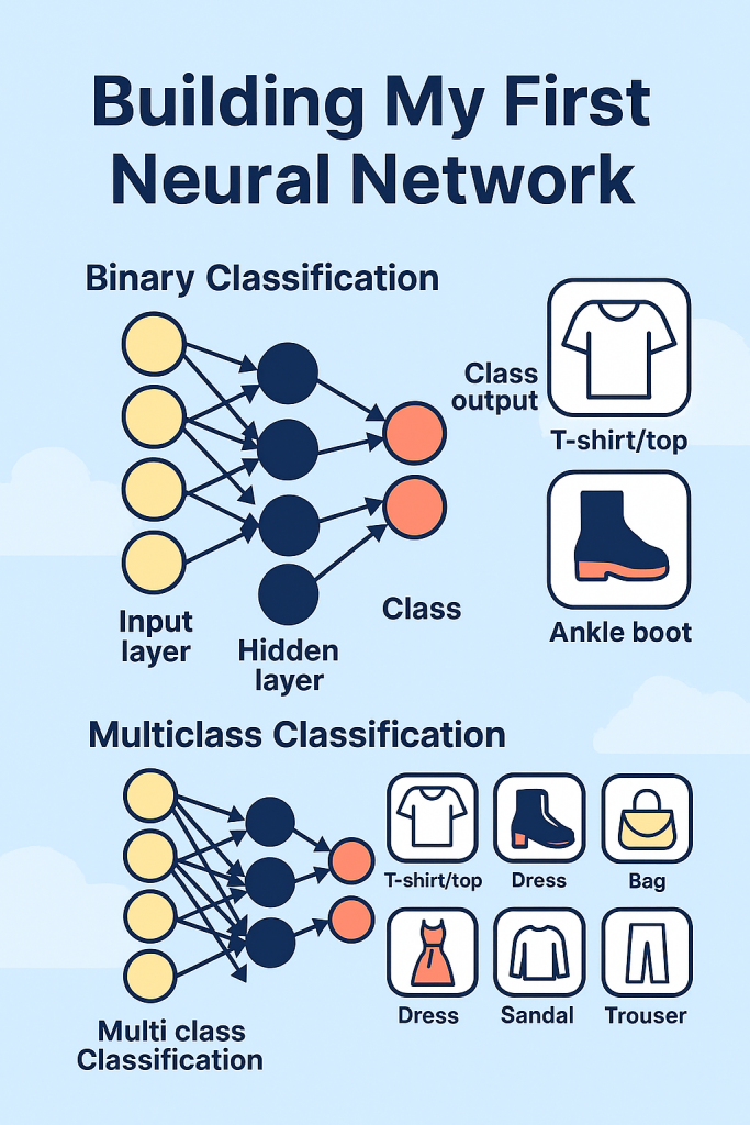
Why Start Here
Transformers are powerful, but at their core they are still neural networks. By practicing with binary and multiclass classification, I can:
- Understand how data flows through a network
- Learn how to define and train models in PyTorch
- Explore loss functions, optimizers, and evaluation metrics
- Build intuition for overfitting, generalization, and early stopping
This hands-on practice will make it easier to understand the more complex architectures later in the series.
What I Built
The notebook I created walks through the entire workflow of training neural networks on FashionMNIST. It includes:
Data Loading and Preprocessing
- Downloading FashionMNIST with
torchvision.datasets - Normalizing images and converting them to tensors
- Visualizing sample images with their labels
Binary Classification
- Filtering the dataset to only two classes: T-shirt/top and Ankle Boot
- Defining a simple multilayer perceptron (MLP)
- Training the model and evaluating accuracy
Multiclass Classification
- Using all 10 classes in the dataset
- Splitting data into training, validation, and test sets
- Defining a deeper MLP with multiple hidden layers
- Implementing modular training and validation functions
- Adding early stopping to prevent overfitting
- Evaluating predictions with accuracy scores and visualizations
Visualization
- Plotting training and validation loss curves
- Displaying sample predictions alongside actual labels
- Highlighting misclassifications to better understand model behavior
Key Concepts Covered
- DataLoader for efficient batching and shuffling
- MLP (Multilayer Perceptron) as the building block of neural networks
- Loss Functions: Binary Cross Entropy for binary classification and Cross Entropy for multiclass classification
- Optimizer: Adam for efficient gradient updates
- Early Stopping to prevent overfitting
- Visualization with matplotlib to interpret results
Results
The models achieved solid accuracy on both binary and multiclass tasks. More importantly, the process gave me a clear understanding of how to structure training loops, monitor performance, and debug issues. Seeing the model correctly classify clothing images was a rewarding first step.
How You Can Try It
You can run the notebook yourself by cloning the repository and installing the dependencies:
pip install torch torchvision matplotlib numpyThen open the notebook in Jupyter or VS Code and run the cells in order. Each section is explained with markdown so you can follow along easily.
👉 View the code on GitHub
Build It Yourself
If you want to try building it yourself, you can find the complete code with detailed explanations of each block in the source code section at the end of this post. All the best!
What’s Next
This was just the beginning. In the next part of the series, I will experiment with Generative Adversarial Networks (GANs) and Variational Autoencoders (VAEs) for image generation.
Then, I will move closer to transformers by exploring attention mechanisms and building a small-scale GPT-like model from scratch. The goal is to gradually increase complexity while keeping the learning process transparent and reproducible.
If you are interested in following along, stay tuned for the next post. I will continue to share code, explanations, and lessons learned as I progress toward building my own open-source transformer model.
Source Code
Import Required Libraries
Import the necessary libraries for building and training a neural network on image data using PyTorch and Torchvision.
torch: Core PyTorch library for tensor operations and neural network building blocks.torch.nn as nn: Provides modules and classes for defining neural network layers and architectures.torchvision: Contains popular datasets, model architectures, and image transformation utilities for computer vision tasks.torchvision.transforms as transforms: Utilities for preprocessing and augmenting image data (e.g., converting to tensors, normalization).%pip install matplotlib: Installs the matplotlib library directly from the notebook if not already present (Jupyter magic command).matplotlib.pyplot as plt: Used for visualizing images, predictions, and training metrics during model development.
These libraries form the foundation for loading data, building models, training, and visualizing results in PyTorch-based computer vision workflows.
import torch
import torch.nn as nn
import torchvision
import torchvision.transforms as transforms
%pip install matplotlib
import matplotlib.pyplot as plt
import numpy as np
Set Random Seed and Define Transform
To ensure reproducibility of results, we set a manual seed so that random operations (like weight initialization and data shuffling) yield the same outcome each run. The transform object defines a sequence of preprocessing steps for the input images:
ToTensor(): Converts images to PyTorch tensors and scales pixel values to [0, 1].Normalize([0.5], [0.5]): Normalizes the tensor so that its mean is 0.5 and standard deviation is 0.5, effectively scaling pixel values to [-1, 1].
This preprocessing is standard for many vision tasks and helps the model train more effectively.
torch.manual_seed(42)
transform = transforms.Compose([
    transforms.ToTensor(),
    transforms.Normalize([0.5],[0.5])
])
Load FashionMNIST Training and Test Datasets
Here we download and prepare the FashionMNIST dataset, a popular benchmark for image classification. FashionMNIST consists of 28×28 grayscale images of 10 clothing categories (such as shirts, trousers, and shoes), with 60,000 training and 10,000 test images.
train_dataset: Loads the training split. If not already present, the dataset will be downloaded to the current directory. Thetransformpipeline defined earlier is applied to each image.test_dataset: Loads the test split, also applying the same transform for consistency.
Parameters explained:
root='.': Store data in the current directory.train=True/False: Selects the training or test split.download=True: Downloads the dataset if not already present.transform=transform: Applies the preprocessing pipeline to each image.
FashionMNIST is a drop-in replacement for the classic MNIST digits dataset, but with more challenging, real-world images. This setup ensures both training and test data are preprocessed identically, which is important for fair evaluation.
train_dataset = torchvision.datasets.FashionMNIST(
    root = '.',
    train = True,
    download = True,
    transform = transform
    )

test_dataset = torchvision.datasets.FashionMNIST(
    root = '.',
    train = False,
    download = True,
    transform = transform
)

print(train_dataset[0])
Define Class Labels for FashionMNIST
The FashionMNIST dataset contains images of clothing items, each labeled with an integer from 0 to 9. To make predictions and visualizations more interpretable, we define a list of human-readable class names corresponding to each label:
- 0: T-shirt/top
- 1: Trouser
- 2: Pullover
- 3: Dress
- 4: Coat
- 5: Sandal
- 6: Shirt
- 7: Sneaker
- 8: Bag
- 9: Ankle Boot
This list, clothes_labels, allows us to map model outputs or dataset labels to their descriptive names, making it easier to display results and understand model performance.
clothes_labels = ['T-shirt/top', 'Trouser', 'Pullover', 'Dress', 'Coat', 'Sandal', 'Shirt', 'Sneaker', 'Bag', 'Ankle Boot']
Visualize Sample Images from the Training Set
This code cell displays a grid of 20 sample images from the FashionMNIST training dataset, along with their corresponding class labels. Visualization is a crucial first step in understanding the dataset and verifying that preprocessing steps (such as normalization and tensor conversion) have been applied correctly.
How it works:
- Creates a figure with high resolution (
dpi=300) and a wide aspect ratio for clear visualization. - Iterates over the first 20 images in the training set.
- For each image:
- Retrieves the image tensor and label.
- Un-normalizes the image (reverses the normalization to bring pixel values back to [0, 1] for display).
- Reshapes the tensor to 28×28 pixels (the original image size).
- Plots the image in grayscale (
cmap='binary'). - Hides axis ticks for a cleaner look.
- Sets the subplot title to the human-readable class name using the
clothes_labelslist.
- Finally, displays the grid of images using
plt.show().
This visualization helps confirm that the data loading and label mapping are correct, and gives an intuitive sense of the variety and difficulty of the classification task.
plt.figure(dpi=300, figsize=(8,4))
for i in range(20):
    ax = plt.subplot(3,8,i+1)
    img = train_dataset[i][0]
    img = img/2 + 0.5
    img = img.reshape(28,28)
    plt.imshow(img, cmap='binary')
    plt.axis('off')
    plt.title(clothes_labels[train_dataset[i][1]], fontsize=6)
plt.show()
Create Binary Classification Datasets (T-shirt/top vs Ankle Boot)
To simplify the classification task, we create new datasets containing only two classes from FashionMNIST:
- Class 0: T-shirt/top
- Class 9: Ankle Boot
How it works:
binary_train_dataset: Contains only training samples where the label is 0 or 9.binary_test_dataset: Contains only test samples where the label is 0 or 9.
This is achieved by filtering the original train_dataset and test_dataset to include only those samples whose label (x[1]) is either 0 or 9.
Why do this?
- Binary classification is often used as a first step to test model performance and debug the pipeline before tackling the full 10-class problem.
- It allows for simpler models and faster experimentation, making it easier to spot issues in data handling or model training.
You can now use these filtered datasets to train and evaluate a model that distinguishes between T-shirts/tops and ankle boots.
binary_train_dataset = [x for x in train_dataset if x[1] in [0,9]]
binary_test_dataset = [x for x in test_dataset if x[1] in [0,9]]
Create DataLoaders for Binary Classification
To efficiently train and evaluate the model, we use PyTorch’s DataLoader to batch and shuffle the binary datasets:
binary_train_loader: Loads batches of samples from the binary training dataset (T-shirt/top vs Ankle Boot), shuffling the data each epoch to improve generalization.binary_test_loader: Loads batches from the binary test dataset, also shuffling for consistency.
Key parameters:
dataset: The filtered dataset containing only the two target classes.batch_size = 32: Number of samples per batch. Larger batches can speed up training but require more memory.shuffle = True: Randomizes the order of samples at the start of each epoch, which helps prevent the model from learning spurious patterns based on data order.
Using DataLoaders allows for efficient mini-batch training, automatic batching, and easy iteration over the dataset during both training and evaluation.
batch_size = 32
binary_train_loader = torch.utils.data.DataLoader(
    dataset = binary_train_dataset,
    batch_size = batch_size,
    shuffle = True
)
binary_test_loader = torch.utils.data.DataLoader(
    dataset = binary_test_dataset,
    batch_size = batch_size,
    shuffle = True
)
Define a Neural Network for Binary Classification
This code cell creates a fully connected neural network (multilayer perceptron) for classifying FashionMNIST images as either T-shirt/top (class 0) or Ankle Boot (class 9).
Architecture details:
- The input layer flattens each 28×28 image into a 784-dimensional vector.
- The network consists of several hidden layers with ReLU activations:
- Linear(784, 512) → ReLU
- Linear(512, 256) → ReLU
- Linear(256, 128) → ReLU
- Linear(128, 64) → ReLU
- Linear(64, 32) → ReLU
- The final output layer is:
- Linear(32, 1): Outputs a single value (logit) for binary classification.
- Dropout(0.25): Randomly zeroes 25% of the outputs during training to help prevent overfitting.
- Sigmoid(): Squashes the output to the [0, 1] range, representing the probability of the image being class 1 (Ankle Boot).
- The model is moved to the appropriate device (
cudaif available, otherwisecpu).
Why this design?
- Multiple hidden layers and nonlinearities allow the model to learn complex patterns in the data.
- Dropout regularization helps the model generalize better to unseen data.
- The final Sigmoid activation is standard for binary classification tasks.
This model is now ready to be trained using a suitable loss function (e.g., BCELoss or BCEWithLogitsLoss) and optimizer.
device = 'cuda' if torch.cuda.is_available() else 'cpu'
binary_classifier = nn.Sequential(
    nn.Linear(28*28,512),
    nn.ReLU(),
    nn.Linear(512,256),
    nn.ReLU(),
    nn.Linear(256,128),
    nn.ReLU(),
    nn.Linear(128,64),
    nn.ReLU(),
    nn.Linear(64,32),
    nn.ReLU(),
    nn.Linear(32,1),
    nn.Dropout(0.25),
    nn.Sigmoid()
).to(device)
Set Training Hyperparameters, Optimizer, and Loss Function
This cell defines the key settings and components needed to train the binary classifier:
learning_rate = 0.001: Controls how much the model weights are updated during each optimization step. A smaller value means slower, more stable learning; a larger value can speed up training but may cause instability.epochs = 50: The number of times the model will iterate over the entire training dataset. More epochs can improve performance but may lead to overfitting if too high.optimizer = torch.optim.Adam(...): Uses the Adam optimizer, which adapts the learning rate for each parameter and generally works well for deep learning tasks. It is initialized with the model’s parameters and the specified learning rate.loss_function = nn.BCELoss(): Binary Cross Entropy Loss is used for binary classification problems. It measures the difference between the predicted probabilities (from the Sigmoid output) and the true binary labels (0 or 1).
These settings and components are essential for training the neural network, controlling how it learns from the data and how performance is measured during training.
learning_rate = 0.001
epochs = 50
optimizer = torch.optim.Adam(binary_classifier.parameters(), lr = learning_rate)
loss_function = nn.BCELoss()
Training Loop for Binary Classifier
This cell implements the main training loop for the binary neural network classifier:
How it works:
- For each epoch (full pass through the training data):
- Initializes
training_lossto accumulate the loss for the epoch. - Iterates over batches from
binary_train_loader:- Flattens each image to a 784-dimensional vector and moves it to the selected device (CPU or GPU).
- Converts labels to float and ensures they are 0 or 1, reshaping to match the model’s output shape.
- Computes predictions using the model.
- Calculates the binary cross-entropy loss between predictions and true labels.
- Clears previous gradients, performs backpropagation, and updates model weights using the optimizer.
- Adds the batch loss to the running total.
- Averages the loss over all batches for the epoch.
- Prints the epoch number and average loss for monitoring training progress.
- Initializes
Why this structure?
- Mini-batch training improves convergence and makes efficient use of hardware.
- Printing the loss each epoch helps track learning and diagnose issues (e.g., if the loss is not decreasing).
This loop is the core of model training, iteratively improving the classifier’s ability to distinguish between T-shirts/tops and ankle boots.
for i in range(epochs):
    training_loss = 0
    for images, labels in binary_train_loader:
        images = images.reshape(-1,28*28).to(device)
        labels = torch.FloatTensor([x if x == 0 else 1 for x in labels])
        labels = labels.reshape(-1,1).to(device)
        predictions = binary_classifier(images)
        loss = loss_function(predictions,labels)
        optimizer.zero_grad()
        loss.backward()
        optimizer.step()
        training_loss += loss.detach()
    training_loss = training_loss/len(binary_train_loader)
    print(f"Epoch: {i} - Loss: {training_loss}")
Evaluate Model Accuracy on Test Set
This cell evaluates the trained binary classifier on the test dataset and computes its accuracy:
How it works:
- Iterates over batches from
binary_test_loader:- Flattens each image to a 784-dimensional vector and moves it to the selected device.
- Converts labels to float and ensures they are 0 or 1, reshaping to match the model’s output shape.
- Computes predictions using the trained model.
- Applies a threshold of 0.5 to the model’s output (from the Sigmoid activation) to obtain binary predictions (0 or 1).
- Compares predicted labels to true labels to determine which predictions are correct.
- Appends the mean accuracy for the batch to the
resultslist.
- After all batches are processed, calculates the overall accuracy as the mean of all batch accuracies.
- Prints the final accuracy as a percentage.
Why this structure?
- Evaluating in batches is memory-efficient and consistent with how the model was trained.
- Using
.detach().cpu().numpy()ensures that accuracy calculations are performed outside the computation graph and on the CPU, which is safer and more efficient for evaluation. - The threshold of 0.5 is standard for binary classification with Sigmoid outputs.
This step provides a quantitative measure of how well the model generalizes to unseen data, which is crucial for assessing real-world performance.
results = []
for images, labels in binary_test_loader:
    images = images.reshape(-1,28*28).to(device)
    labels = torch.FloatTensor([x if x == 0 else 1 for x in labels])
    labels = labels.reshape(-1,1).to(device)
    predictions = binary_classifier(images)
    binary_predictions = torch.where(predictions > 0.5, 1, 0)
    correct_predictions = (binary_predictions == labels)
    results.append(correct_predictions.detach().cpu().numpy().mean())
accuracy = np.array(results).mean()
print(f"Accuracy: {accuracy*100}%")
Split Training Data and Create DataLoaders for Multiclass Classification
This cell prepares the data for multiclass (10-class) classification by splitting the original training set and creating DataLoaders for training, validation, and testing:
How it works:
- Splits the original
train_datasetinto two subsets:train_dataset: 50,000 samples for training.validation_dataset: 10,000 samples for validation (to monitor model performance and tune hyperparameters).- This is done using
torch.utils.data.random_split, which randomly partitions the dataset.
- Creates DataLoaders for each subset:
multi_train_loader: Loads batches from the training set, shuffling each epoch for better generalization.multi_validation_loader: Loads batches from the validation set, also shuffling.multi_test_loader: Loads batches from the test set, shuffling for consistency.
- All DataLoaders use the same
batch_sizeas before.
Why this structure?
- Splitting the data allows for unbiased evaluation of the model during training (validation) and after training (test).
- DataLoaders enable efficient mini-batch training and evaluation, which is essential for deep learning workflows.
This setup is a standard best practice for training robust and generalizable neural networks on image classification tasks.
train_dataset, validation_dataset = torch.utils.data.random_split(train_dataset, [50000,10000])

multi_train_loader = torch.utils.data.DataLoader(
    dataset = train_dataset,
    batch_size = batch_size,
    shuffle = True
)
multi_validation_loader = torch.utils.data.DataLoader(
    dataset = validation_dataset,
    batch_size = batch_size,
    shuffle = True
)
multi_test_loader = torch.utils.data.DataLoader(
    dataset = test_dataset,
    batch_size = batch_size,
    shuffle = True
)
Early Stopping Utility Class
This cell defines an EarlyStop class, a utility for implementing early stopping during model training. Early stopping is a regularization technique used to prevent overfitting by halting training when the model’s performance on a validation set stops improving.
How it works:
__init__(self, patience=10): Initializes the class with apatienceparameter (default 10). Patience is the number of consecutive epochs to wait for an improvement in validation loss before stopping training.self.steps: Counts the number of epochs since the last improvement in validation loss.self.best_loss: Tracks the lowest validation loss seen so far.stop(self, current_loss):- If the current validation loss is lower than
best_loss, updatesbest_lossand resetsstepsto 0. - If not, increments
stepsby 1. - If
stepsreaches or exceedspatience, returnsTrueto signal that training should stop; otherwise, returnsFalse.
- If the current validation loss is lower than
Why use early stopping?
- Prevents overfitting by stopping training once the model stops improving on the validation set.
- Saves computational resources by avoiding unnecessary epochs.
- Commonly used in deep learning workflows for robust model selection.
To use this class, instantiate it before training and call stop(validation_loss) at the end of each epoch. If it returns True, halt training.
class EarlyStop:
    def __init__(self, patience=10):
        self.patience = patience
        self.steps = 0
        self.best_loss = float('inf')
    def stop(self, current_loss):
        if current_loss < self.best_loss:
            self.best_loss = current_loss
            self.steps = 0
        elif current_loss >= self.best_loss:
            self.steps += 1
        if self.steps >= self.patience:
            return True
        else:
            return False

early_stopper = EarlyStop()
Define a Neural Network for Multiclass Classification
This cell creates a fully connected neural network (multilayer perceptron) for classifying FashionMNIST images into one of 10 clothing categories.
Architecture details:
- The input layer flattens each 28×28 image into a 784-dimensional vector.
- The network consists of several hidden layers with ReLU activations:
- Linear(784, 512) → ReLU
- Linear(512, 256) → ReLU
- Linear(256, 128) → ReLU
- Linear(128, 64) → ReLU
- The final output layer is:
- Linear(64, 10): Outputs a vector of 10 values (logits), one for each class.
- No activation function is applied to the output layer here, as the standard practice for multiclass classification in PyTorch is to use
nn.CrossEntropyLossduring training, which internally appliesLogSoftmax.
Why this design?
- Multiple hidden layers and nonlinearities allow the model to learn complex patterns in the data.
- The output layer produces raw scores (logits) for each class, which are converted to probabilities during loss calculation or evaluation.
This model is now ready to be trained for multiclass classification using a suitable loss function (e.g., CrossEntropyLoss) and optimizer.
multi_classifier = nn.Sequential(
    nn.Linear(28*28,512),
    nn.ReLU(),
    nn.Linear(512,256),
    nn.ReLU(),
    nn.Linear(256,128),
    nn.ReLU(),
    nn.Linear(128,64),
    nn.ReLU(),
    nn.Linear(64,32),
    nn.ReLU(),
    nn.Linear(32,10)
).to(device)
Set Hyperparameters, Optimizer, and Loss Function for Multiclass Classifier
This cell defines the key training components for the multiclass neural network classifier:
learning_rate = 0.001: Sets the step size for updating model weights during optimization. A smaller value leads to slower, more stable learning; a larger value can speed up training but may cause instability.optimizer = torch.optim.Adam(multi_classifier.parameters(), lr = learning_rate): Uses the Adam optimizer, which adapts the learning rate for each parameter and generally works well for deep learning tasks. It is initialized with the model’s parameters and the specified learning rate.loss_function = nn.CrossEntropyLoss(): Cross Entropy Loss is the standard loss function for multiclass classification. It combinesLogSoftmaxandNLLLossin one class, measuring the difference between the predicted class probabilities (logits) and the true class labels (integers 0-9).
Why these choices?
- Adam optimizer is robust and efficient for most neural network training tasks.
- Cross Entropy Loss is appropriate for problems where each input belongs to exactly one of several classes.
These settings are essential for training the multiclass classifier, controlling how it learns from the data and how performance is measured during training.
learning_rate = 0.001
optimizer = torch.optim.Adam(multi_classifier.parameters(), lr = learning_rate)
loss_function = nn.CrossEntropyLoss()
Training Function for One Epoch (Multiclass Classifier)
This cell defines a function, multi_training_epoch, that performs one full training epoch for the multiclass neural network classifier:
How it works:
- Initializes
training_lossto accumulate the total loss for the epoch. - Iterates over batches from
multi_train_loader:- Flattens each image to a 784-dimensional vector and moves it to the selected device (CPU or GPU).
- Reshapes labels to a 1D tensor (required by
CrossEntropyLoss). - Computes predictions (logits) using the model.
- Calculates the cross-entropy loss between predictions and true labels.
- Clears previous gradients, performs backpropagation, and updates model weights using the optimizer.
- Adds the batch loss to the running total.
- After all batches, averages the loss over the number of batches (
n). - Returns the average training loss for the epoch.
Why use this structure?
- Encapsulating the training logic in a function makes the code modular and reusable for each epoch.
- Mini-batch training improves convergence and makes efficient use of hardware.
- Returning the average loss allows for easy monitoring of training progress.
This function is typically called once per epoch in a training loop to iteratively improve the model’s performance on the training data.
def multi_training_epoch():
    training_loss = 0
    for n, (images, labels) in enumerate(multi_train_loader):
        images = images.reshape(-1,28*28).to(device)
        labels = labels.reshape(-1,).to(device)
        predictions = multi_classifier(images)
        loss = loss_function(predictions, labels)
        optimizer.zero_grad()
        loss.backward()
        optimizer.step()
        training_loss += loss.detach()
    training_loss = training_loss/n
    return training_loss
Validation Function for One Epoch (Multiclass Classifier)
This cell defines a function, multi_validation_epoch, that evaluates the multiclass neural network classifier on the validation set for one epoch:
How it works:
- Initializes
validation_lossto accumulate the total loss for the epoch. - Iterates over batches from
multi_validation_loader:- Flattens each image to a 784-dimensional vector and moves it to the selected device (CPU or GPU).
- Reshapes labels to a 1D tensor (required by
CrossEntropyLoss). - Computes predictions (logits) using the model.
- Calculates the cross-entropy loss between predictions and true labels.
- Adds the batch loss to the running total.
- After all batches, averages the loss over the number of batches (
n). - Returns the average validation loss for the epoch.
Why use this structure?
- Separating validation logic from training ensures that model parameters are not updated during evaluation.
- Monitoring validation loss helps detect overfitting and guides early stopping.
- Returning the average loss allows for easy comparison with training loss and tracking model generalization.
This function is typically called at the end of each training epoch to assess how well the model is performing on unseen validation data.
def multi_validation_epoch():
    validation_loss = 0
    for n, (images, labels) in enumerate(multi_validation_loader):
        images = images.reshape(-1, 28*28).to(device)
        labels = labels.reshape(-1,).to(device)
        predictions = multi_classifier(images)
        loss = loss_function(predictions, labels)
        validation_loss += loss.detach()
    validation_loss = validation_loss/n
    return validation_loss
Training Loop with Early Stopping for Multiclass Classifier
This cell implements the main training loop for the multiclass neural network classifier, incorporating early stopping based on validation loss:
How it works:
- Sets
max_epochs = 100as the maximum number of training epochs. - For each epoch:
- Calls
multi_training_epoch()to perform one full pass over the training data and returns the average training loss. - Calls
multi_validation_epoch()to evaluate the model on the validation set and returns the average validation loss. - Calls
early_stopper.stop(validation_loss)to check if validation loss has not improved for a specified number of epochs (patience). If so, early stopping is triggered. - If early stopping is triggered, prints a message and breaks the loop.
- Otherwise, prints the current epoch, training loss, and validation loss for monitoring progress.
- Calls
Why use this structure?
- Early stopping helps prevent overfitting by halting training when the model stops improving on the validation set, saving time and computational resources.
- Monitoring both training and validation loss provides insight into model learning and generalization.
- Printing progress each epoch allows for real-time tracking and debugging.
This loop is the core of model training, ensuring the model learns effectively while avoiding overfitting through early stopping.
max_epochs = 100
for i in range(max_epochs):
    training_loss = multi_training_epoch()
    validation_loss = multi_validation_epoch()
    print(f"Epoch: {i+1} - Training Loss: {training_loss} - Validation Loss: {validation_loss}")
    early_stop = early_stopper.stop(validation_loss)
    if early_stop:
        print(f"Early Stop at epoch {i+1} with validation loss {validation_loss}")
        break
Visualize Test Images and Model Predictions (Multiclass Classifier)
This cell provides both a visual and textual evaluation of the trained multiclass classifier on the FashionMNIST test set:
1. Visualizing Test Images
- Displays the first 10 images from the test dataset in a 2×5 grid.
- Each image is un-normalized (reversing the earlier normalization) and reshaped to its original 28×28 pixel format for display.
- The subplot title shows both the human-readable class name and the corresponding label index (e.g., “Sneaker-7”).
- This visualization helps confirm that the test data is correctly formatted and provides a quick look at the variety of classes.
2. Printing Actual vs. Predicted Labels
- For each of the first 10 test images:
- The image is reshaped and moved to the appropriate device (CPU or GPU).
- The trained multiclass classifier predicts the logits for all 10 classes.
torch.argmax(prediction)selects the class with the highest predicted score as the model’s output.- Both the actual label and the predicted label are printed, along with their human-readable class names from
clothes_labels.
- This textual output allows you to directly compare the model’s predictions to the ground truth, making it easy to spot correct and incorrect classifications.
Why is this important?
- Visual and textual inspection of predictions is a key step in model evaluation, helping to identify strengths and weaknesses that may not be apparent from accuracy metrics alone.
- It can reveal systematic errors (e.g., confusing similar classes) and help guide further model improvements.
This cell is a practical way to qualitatively assess the model’s performance and gain intuition about its decision-making on real test images.
plt.figure(dpi=300, figsize=(8,4))
for i in range(10):
    plt.subplot(2,5,i+1)
    image = test_dataset[i][0]
    image = image/2 + 0.5
    image = image.reshape(28,28)
    label = test_dataset[i][1]
    plt.imshow(image, cmap='binary')
    plt.axis('off')
    plt.title(clothes_labels[label] + f"-{label}", fontsize=6)
plt.show()

for i in range(10):
    image = test_dataset[i][0]
    image = image.reshape(-1, 28*28).to(device)
    actual_label = test_dataset[i][1]
    prediction = multi_classifier(image)
    predicted_label = torch.argmax(prediction).item()
    print(f"Actual Label: {actual_label} - {clothes_labels[actual_label]}. Predicted Label: {predicted_label} - {clothes_labels[predicted_label]}.")
Evaluate Multiclass Classifier Accuracy on Test Set
This cell evaluates the trained multiclass neural network classifier on the FashionMNIST test dataset and computes its overall accuracy:
How it works:
- Iterates over batches from
multi_test_loader:- Each batch of images is flattened to 784-dimensional vectors and moved to the appropriate device (CPU or GPU).
- Labels are reshaped to a 1D tensor to match the expected input for accuracy calculation.
- The model predicts logits for all 10 classes for each image in the batch.
torch.argmax(predictions, dim=1)selects the class with the highest predicted score for each image, producing the predicted class labels.- Compares the predicted labels to the true labels to determine which predictions are correct.
- The mean accuracy for the batch is appended to the
resultslist.
- After all batches are processed, calculates the overall accuracy as the mean of all batch accuracies.
- Prints the final accuracy as a percentage.
Why this structure?
- Evaluating in batches is memory-efficient and consistent with how the model was trained.
- Using
.detach().cpu().numpy()ensures that accuracy calculations are performed outside the computation graph and on the CPU, which is safer and more efficient for evaluation. torch.argmaxis standard for converting logits to class predictions in multiclass classification tasks.
What does this tell us?
- The final accuracy value provides a quantitative measure of how well the trained model generalizes to unseen data across all 10 clothing categories.
- High accuracy indicates good model performance, while low accuracy may suggest underfitting, overfitting, or issues with the data or model architecture.
This step is essential for assessing the real-world effectiveness of the multiclass classifier and comparing its performance to other models or approaches.
results = []
for images, labels in multi_test_loader:
    images = images.reshape(-1, 28*28).to(device)
    labels = labels.reshape(-1,).to(device)
    predictions = multi_classifier(images)
    predicted_labels = torch.argmax(predictions, dim=1)
    correct_predictions = (predicted_labels == labels)
    results.append(correct_predictions.detach().cpu().numpy().mean())
accuracy = np.array(results).mean()
print(f"Accuracy: {accuracy*100}%")
Leave a Reply